Can Microsoft Excel formulas be easy to learn? Yep! This tutorial explains the very basics of Excel formulas for beginners, with detailed steps on how to write and use them. It also provides a number of advanced formula examples for experienced users. You will be amazed how simple creating formulas in Excel actually is.
If asked what Microsoft Excel is about, what would be your answer? Right, it's all about storing and crunching numbers. You can use Excel to calculate percentages and compound interest, count and sum cells based on specific criteria, find average, and even get a sample deviation of a given set of values. All this can be done by using Excel formulas.
In this tutorial, we are going to learn the basics of creating and using formulas in Excel. And because one of the most efficient ways to learn is through practice, we will also discuss a number of formulas examples to make things easier to understand. Here's a list of topics we are going to cover:
Microsoft Excel formulas - the basics
In MS Excel, formulas are equations that perform various calculations in your worksheets. Though Microsoft has introduced a handful of new functions over the years, the concept of Excel spreadsheet formulas is the same in all versions of Excel 2016, Excel 2013, Excel 2010, Excel 2007 and lower.
- All Excel formulas begin with an equal sign (=).
- After the equal symbol, you enter either a calculation or function. For example, to add up values in cells B1 through B5, you can either:
- Type the entire equation:
=B1+B2+B3+B4+B5 - Use the SUM function:
=SUM(B1:B5)
- Type the entire equation:
- Press the Enter key to complete the formula. Done!
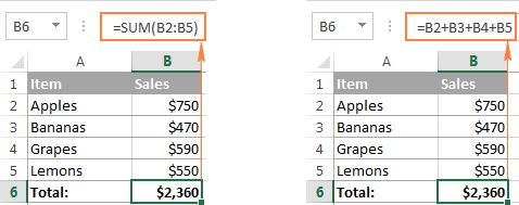
Elements of Microsoft Excel formulas
When you make a formula in Excel, you can use different elements to supply the source data to the formula and indicate what operators should be performed on those data. Depending on the formula type that you create, it can include any or all of the following parts:
- Constants - numbers or text values that you enter directly in a formula, like =2*3.
- Cell references - reference to a cell containing the value you want to use in your Excel formula, e.g.
=SUM(A1, A2, B5).To refer to data in two or more contiguous cells, use a range reference like A1:A5. For example, to sum values in all cell between A1 and A5, inclusive, use this formula:
=SUM(A1:A5). - Names - defined name for a cell range, constant, table, or function, for example
=SUM(my_name). - Functions - predefined formulas in Excel that perform calculations using the values supplied in their arguments.
- Operators - special symbols that specify the type of operation or calculation to be performed.
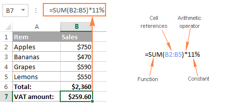
Operators in Excel worksheet formulas
To tell Microsoft Excel what type of operation you want to perform in a formula, you use special symbols that are technically called operators. There exist 4 types of operators in Excel:
- Arithmetic - to perform basic mathematical operations.
- Comparison (logical) - to compare values.
- Concatenation - to join text values into a single string.
- Reference - to make ranges and separate arguments in Excel functions.
Using arithmetic operators in Excel formulas
These operators are used to perform basic mathematical operations such as addition, subtraction, multiplication, and division.
| Operator | Meaning | Formula example |
| + (plus sign) | Addition | =A2+B2 |
| - (minus sign) | Subtraction Negation (reversing the sign) |
=A2-B2=-A2 (changes the sign of the value in A2) |
| * (asterisk) | Multiplication | =A2*B2 |
| / (forward slash) | Division | =A2/B2 |
| % (percent sign) | Percentage | =A2*10%(returns 10% of the value in A2) |
| ^ (caret) | Exponential (power of) | =A2^3(raises the number in A2 to the power of 3) |
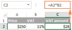
For example, if you have an item price in cell A2 and VAT in cell B2, you can calculate the VAT amount by using the following percentage formula: =A2*B2
Comparison operators in Excel formulas
In Microsoft Excel formulas, comparison, or logical, operators are used to compare two values. The result of the comparison is always a logical value of TRUE or FALSE. The following logical operators are available in Excel:
| Comparison operator | Meaning | Formula example |
| = | Equal to | =A2=B2 |
| <> | Not equal to | =A2<>B2 |
| > | Greater than | =A2>B2 |
| < | Less than | =A2<B2 |
| >= | Greater than or equal to | =A2>=B2 |
| <= | Less than or equal to | =A2<=B2 |
For example, formula =A1=B1 returns TRUE if cells A1 and B1 contain the same value (number, text or date), FALSE otherwise.
For more information and examples of using comparison operators in MS Excel formulas, please check out the following tutorial: Excel logical operators - equal to, not equal to, greater than, less than.
Text concatenation operator
Text concatenation operator in Excel is the ampersand symbol (&). You can use it to join two or more text strings in a single string.
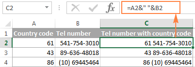
For example, if you have country codes in column A and telephone numbers in column B, you can use the following formula to get the telephone numbers combined with the country codes:
=A1&" "&B1
In the above formula, we concatenate a space " " in between to make the numbers better readable:
The same result can be achieved by using the CONCATENATE function, and the following tutorial explains all the details: How to combine text strings, cells and columns in Excel.
Reference operators in Excel formulas and functions
To supply ranges to MS Excel formulas and separate arguments in Excel functions, the following operators are used.
Colon (:) - it is a range operator that allows you to make one reference for multiple cells located between 2 cells that you specify.
For example, range A1:A00 includes 100 cells from A1 through A100. To find an average of those 100 cells, you use the following formula:
=AVERAGE(A1:A00)
You can also refer to the entire column (A:A) or the entire row (1:1). For example, the following formula finds the total of all numbers in column A: =SUM(A:A). Find more about whole-column and whole-row references.
Comma (,) - is used to separate arguments in Excel spreadsheet formulas. For example, the formula =IF(A1>0, "good", "bad") reads as follows: if A1 is greater than zero, return "good", otherwise "bad".
Note. Comma is the default List Separator in North America and some other countries. In European countries, comma is reserved as the Decimal Symbol and the List Separator is usually set to semicolon (;). In this case, you need to separate a function's arguments with semicolons, e.g.
=IF(A1>0; "good"; "bad")
So, if you are trying to make a formula in your worksheet, but Excel does not accept it and throws up an "invalid formula" error, go to your Regional Settings (Control Panel > Region and Language > Additional Settings) and check what symbol is set as List Separator there. It is that symbol that you need to use to separate arguments in your Excel formulas.
Space - it is an intersection operator that lets you get the cell(s) common to the two references that you specify. For example, if you a list of items in column A and some related data in other columns, you can get a value at the
intersection of a given column and row by using a formula like this:
=B3:D3 C2:C4

For a real-life formula example, see how you can do two-way lookup in Excel by using named ranges & space operator.
Excel formula types
Formulas that you create in your Excel spreadsheets can be simple or complex:
- Simple Excel formulas perform just one mathematical operation, for example
=10*5or=SUM(A1:A10) - Complex (advanced) Excel formulas include more than one calculation, for example
=10*5+20or=SUM(A1:A10)/2
Further on in this tutorial, you will find the detailed steps for making both types of Excel spreadsheet formulas.
How to create formulas in Excel
As already mentioned, any Excel formula starts with the equal sign (=). So, whatever formula you are going to write, begin by typing = either in the destination cell or in the Excel formula bar. And now, let's have a closer look at how you can make different formulas in Excel.
How to create simple formulas in Excel
Although simple Excel formulas perform just one calculation, they can do this in many different ways. You can supply the source data as constants, cell references, or defined names, and perform calculations by using mathematical operators or Excel functions. For detailed steps, please see the following resources:
How to create advanced formulas in Excel
When you have some experience with simple Excel formulas, you may want to perform several calculations within a single formula. And the following examples show how you can do this.
Creating complex formulas with constants and mathematic operators
For a complex Excel formula to calculate correctly, certain operations must be performed before others. The default order of operations in Excel formulas is this:
- Mathematical operations enclosed in parenthesis
- Power of (exponential calculations)
- Multiplication and division, whichever comes first in a formula
- Addition and subtraction, whichever comes first in a formula
For example, you can use the following formulas to calculate the total and commission:

And now, let's break down these formulas to see how Microsoft Excel calculates them:
Total formula: =$B2*$D2+$B2*$D2*$C2
- 1st multiplication: $B2*$D2 (price*qty. = amount)
- 2nd and 3rd multiplications: $B2*$D2*$C2 (price*qty.*VAT % = VAT amount)
- Addition: amount + VAT amount = total
Commission formula: =($B2*$D2+$B2*$D2*$C2)*10%
To calculate the 10% commission, you need to multiply the total by 10%, so you enclose the previous calculation in brackets, and got the result you want.
Of course, nothing prevents you from multiplying the total already calculated in column E by 10%, in this case the formula would reduce to a simple calculation =E2*10%. However, in large worksheets, it makes sense to write independently calculated formulas, so that removing a column with one formula wouldn't break the others.
Excel formulas with nested functions
In Microsoft Excel formulas, nesting one function within another means using one function as an argument of another function. In modern versions of Excel 2016, 2013, 2010 and 2010, you can use up to 64 nested functions. In older versions of Excel 2003 and lower, only up to 7 levels of functions are allowed.
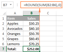
Here is a very simple example of a nested Excel formula that includes the SUM function to find the total, and ROUND function to round that number to the nearest integer (0 decimal places):
=ROUND(SUM(B2:B6),0)
Of all Excel functions, IF is nested more often than all others. As you probably know, the IF function is used to evaluate a specified condition and return one value when condition is met, and another value when the condition is not met. However, quote often you have to deal with situations where there are more than two possible outcomes. And if this case, you can write several IF functions and nest them into each other:
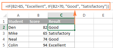
For the detailed explanation of nested IF's syntax and advanced formula examples, please check out the following tutorial: Using nested IF functions in Excel.
Array formulas in Excel
Array formulas in Excel are advanced aerobatics. A single Excel array formula can perform thousands of calculations and replace hundreds of usual formulas. Learning array formulas certainly requires some time and effort, but it's worth it.
Since this tutorial is purposed for beginners, I won't intimidate you by the definitions of array constants and complex multi-line formulas. I'll show just one very simple example of an Excel array formula that demonstrates what they are capable for.
Supposing you have 2 columns of numbers, column A and B. And you want to know how many times column B is greater than or equal to column A when a value in column B is greater than 0.
This task requires comparing two ranges and you can do this by using the following array formula:
=SUM((B2:B10>=A2:A10) * (B2:B10>0))
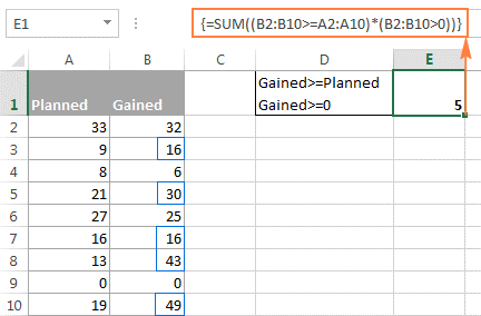
Note. To enter an Excel array formula correctly, you have to press Ctrl+Shift+Enter instead of conventional Enter stroke.
To learn more about Excel array formulas, please see the following tutorials:
- Excel array formulas, functions and constants - explains the basics of array formulas and shows how to use array constants and array functions.
- Excel array formula examples for beginners and power users - 7 fascinating examples of advanced array formulas in Excel.
Excel user defined functions
Although Microsoft Excel has hundreds of built in functions, you still may find yourself faced with a challenge for which no predefined Excel function exists. In this case, you can create that function yourself... or have somebody create it for you :)
Such custom functions are called User Defined Functions (UDFs), and they are especially useful for advanced mathematic or engineering calculations. Like macros, user defined functions are written in VBA (Visual Basic for Applications). As an example, you can review and download custom functions created by our team to count and sum cells by color.
Absolute, relative and mixed cell references in Excel formulas
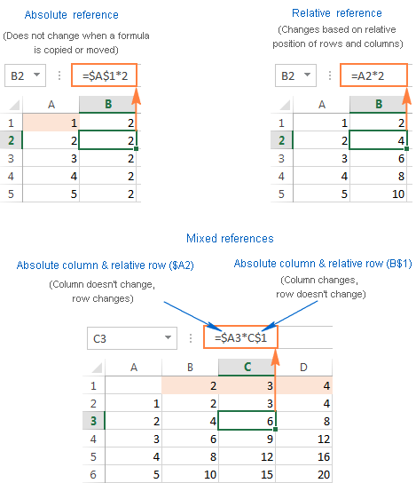
There exist 3 types of cell references in Excel: absolute ($A$1), relative (A1) and mixed ($A1 or A$1). All three of the above references refer to the same cell, and the dollar sign ($) is used only for one purpose - it tells Microsoft Excel whether to change or not to change cell references when the formula is moved or copied to other cells.
Absolute cell reference ($A$1) - the $ sign before the row and column coordinates makes a reference static, and lets you copy a formula without changing references.
Relative cell reference (A1) - a cell reference with no $ sign changes based on relative position of rows and columns in a spreadsheet.
Mixed cell reference - can be of 2 types:
- Absolute column and relative row ($A1) - the $ sign in front of the column letter locks the reference to the specified column, so the column never changes. The relative row reference, without the dollar sign, changes depending on the row to which the formula is copied.
- Relative column and absolute row (A$1) - the row's reference locked by $ doesn't change, and the column's reference does.
The following image shows how different reference types work in practice.
For more information about Excel cell reference and more formula examples, please see Why use $ in Excel formulas.
Tips and time-saving shortcuts for Excel formulas
Formulas in Excel are a powerful multi-faceted tool, and they can solve a great variety of tasks in your spreadsheets. Of course, learning various aspects of Microsoft Excel formulas and functions does take time, so you might feel there isn't enough time in the day to learn everything. Well, a good way to find more time is to save some time :)
- To toggle between absolute, relative and mixed references in a formula, use the F4 key as demonstrated in Switching between reference types in Excel.
- To view all formulas on the sheet, click the Show formulas button on the Formulas tab > Formula Auditing group or press the Ctrl+~ shortcut.
- To edit a formula, press F2, or double click a cell, or click the formula bar.
- To debug formulas in Excel, select a formula part and press F9. This will let you see the actual values behind cell references.
- To copy a formula to all cells in a column, enter the formula in the first cell, select that cell, and hover the cursor over the small square in bottom right corner until it changes to a black cross (which is called
the fill handle). Double click that cross, and you will get the formula copied through the entire column. - To convert formulas to values, select all cells with formulas that you want to convert, press Ctrl+C to copy those formulas, then press Shift+F10, then press V, and then hit Enter. Shift + F10 + V is the shortcut for Excel's Paste special - values only. If you are not sure you will remember this shortcut, then simply press a usual shortcut for paste Ctrl+V, click the small arrow to the right of the Paste button to open the drop-down list, and select Paste Values. For more information, see How to replace formulas with their values in Excel.
Microsoft Excel formulas with examples
Excel provides formulas for almost anything, and there exist tens or even hundreds of different functions in modern versions of Microsoft Excel. So, if you encounter a task for which you cannot work out a solution, most likely you are missing out on a formula that can do it for you. Before spending hours and hours on performing manual calculations, take a few minutes to review the following resources. It is a selection of the most popular MS Excel formulas with examples, grouped by categories.
Excel percentage formula
Excel sum formulas
Count formula in Excel
Average formula in Excel
Excel date formulas
Time formulas in Excel
Excel formulas for VLOOKUP
Excel conditional formatting formulas
Well, we seem to have finally got to the end. What was planned as a short Excel formula tutorial for beginners has nearly turned into a voluminous manual because there are so many different aspects of Excel formulas to cover. I am really thankful to everyone who has read this page to the end!
 by
by
95 comments
I like it
Hi
I need help on the excel formula. vlookup and match.
Hi! Detailed instructions and examples of the VLOOKUP and MATCH functions can be found in these articles: Excel VLOOKUP function tutorial with formula examples and Excel MATCH function with formula examples, Excel INDEX MATCH vs. VLOOKUP.
3+6+3+5+5
i want to total this numbers in another cell, if i changes like 3+6+3+5+5+6+7 means it should be add automatically if and possible to solve the formula .
Hi! You can convert text into a Excel formula using VBA.
please is max and min a formula or function
Hi! I recommend reading these guides: Excel MAX function - formula examples to find highest value and How to use MIN function in Excel.
Hi, what formula should I use if I want to know the expected date and time for account due excluding lunch break, after office hour, weekends and holidays? Thank you
Cell reference:
A1: Start Date and Time - Feb 08, 2024 16:00
B1: Duration - 5 hrs
C1: Lunch break duration - 12:00 to 13:00
D1: Office hours start- 8:30
E1: Office hours end - 17:30
with holiday
A1: Start Date and Time - Dec 31, 2023 16:00
B1: Duration - 5 hrs
C1: Lunch break duration - 12:00 to 13:00
D1: Office hours start- 8:30
E1: Office hours end - 17:30
- office will resume on Jan 2 2024
Hi! A similar question has already been asked here. I hope it’ll be helpful.
I have multiple GL codes and I'm not sure which formula I would need, what I want is if I put in code "5320" the next column says "food supply" but if I input "5330" it says "soft supply" ect for each code. Basically I want to put in the code and the next column auto fills with the correct gl name for that code.
Hi! Create a special table in which each code corresponds to its name. You will be able to extract the correct name that matches the code using the VLOOKUP function. We have a special tutorial on this. Please see: Excel VLOOKUP function tutorial with formula examples.
My formula, =IF(C4=Results!C5,1)+IF(C4=Results!D5,2)+IF(C4=Results!E5,3) works well but shows the number 6 in C5 when sheet Results!C5 D5 and E5 are empty. How can I get rid of the Number 6 and show a blank? Thanks,
Hi! Add another IF function to your formula to check with the ISBLANK function if the cells are empty. Here is the article that may be helpful to you: Nested IF AND in Excel. If my understanding is correct, the following formula should work for you:
=IF(AND(ISBLANK(Results!C5),ISBLANK(Results!D5),ISBLANK(Results!E5)),"", IF(C4=Results!C5,1)+IF(C4=Results!D5,2)+IF(C4=Results!E5,3))
Hi Alexander,
So many thanks for your prompt and excellent reply. The sheets now work well. I will read up on the nested IF AND so that I may understand this better
Steve Walker
hi I'm trying to create a formula to create a calculator to work out when a specific size is typed in, it multiples the amount specified to that size inputted however the sizes are ranges e.g. 11-20 is £16 so if the product is 18 that mean18x£16 or 21 will times that by another figure I have 10 different price ranges and 10 different sizes ranges from 1-2, 3-5, 6-10, 11-20, 21-50, 51-100, 101-500, 500+, 4-10no. and 11-20no.
Thanks
Hi! Use the IFS logical function for multiple conditions. You can find the examples and detailed instructions here: The new Excel IFS function instead of multiple IF. For example,
=IFS(A1>500,B1*100,A1>101,B1*50,A1>51,B1*20,......)
When am using Excel in business how can I set for the weekly sales to be in one sheet by making sure the tock will continue change according to the daily sales
Please ask a specific question on the Excel formula, provide the source data and the desired result.
Hello,
My question is in my marksheet, i can't get percentage when I started calculate percentage there where show 4500% how is this possible please help me
Hi!
I recommend reading this guide: How to calculate percentage in Excel - formula examples.
I fetched a few values using LOOKUP function and I'm getting #N/A in some of the cells. I've checked the references and the format also the value does exist. I can't see a reason why N/A is showing up even after having all conditions met. Pls help. Others in my team had the same data and they got it using the same formula. Is there a problem in my excel or ...?
VLOOKUP should never be used in modern versions of Excel. Use XLOOKUP instead, or INDEX-MATCH for backwards compatability. VLOOKUP falsely marks many cells as precedents, breaks if a column is inserted or removed between the lookup column and return column, and can't return a value from a column to the left of the lookup column.
Hello!
See this article for all the possible causes of your problem and their solution: Excel VLOOKUP not working - solving #N/A and #VALUE errors. This should solve your task.
I am trying to write a formula for correctly guessing 5 football team positions after a nominated period. My sheet has the 5 positions 1 to 5 in rows 82 to 86, the correct positions are in column U, the guesses are in column W and the points scored are in column X. The formula in column X would return 3 if the guess was correct, 1 if in any of the other 4 positions or 0 if not in any of the 5 positions. I realise all 5 rows would have a slightly different formula. Can you help please?
Hello!
To match a value in a column, use the MATCH function. Use the nested IF function to select a match option.
=IF(U82=W82,3, IF(ISNUMBER(MATCH(W82,$U$82:$U$86,0)),1,0))
Hope this is what you need.
I'm trying to write a formula that will solve this equation for "b" but I don't know how to do it. I've tried several different ways but nothing will give me the correct answer. Please help!
35 = -65.2*0.75+b
Hi!
You just need to remember the mathematics from school.
=35+65.2*0.75
i have a problem my work is on printing large Lonas
anyway how can i make a calculation to calculate the meter square of any product by only putting the price
Hi!
Perhaps the VLOOKUP function will be useful to solve your problem and find the necessary values. If this does not suit you, explain the problem in more detail.
How would I calculate this equation in terms of x and y; when X=1(C5) and Y=3(C6)
4 + y/(2x+y)sqrt 2 + 12
(The 2x+y is in parenthesis but then squared but didn’t know how to type that here.
I just need a formula to get the correct answer. I’ve tried several different ways and I keep getting the incorrect answer.
Hello!
You did not write what result you wanted to get. But I think this formula will work for you -
=4+C6/(2*C5+C6)^2+12
how to convert this 2.1291912051718E-87 to number in excel
Hello!
A number in Excel cannot contain more than 15 digits. Use the rounding functions for numbers.
If your number is written as text, take a look at this article: Convert text to number with formula and other ways.
I hope I answered your question.
I don't really know, but near the top of the page there are two spots that talk about "rages" is that a typo?
**Reference - to make rages and separate arguments in Excel functions.**
Thank you, Ebhe! That's definitely a typo - fixed.
The formula means that if the code entered in cell C5 is equal to cell A14, cell D5 will indicate Baguio, if equal to cell A15, cell D5 will indicate Davao, if equal to cell A16, cell D5 will indicate Cebu...
Can someone help me with this? I need to know what formula should i use... Please...
Hello!
Please check out the following article on our blog, it’ll be sure to help you with your task: Excel Nested IF statements
what does this symbol mean - "*:*"
For example - =COUNTIFS('SCHEDULE '!K:K,"*:*",'SCHEDULE '!$A:$A,$B$78)
Hi Sam,
In Excel, an asterisk (*) is a wildcard that represents any sequence of characters. In your case, "*:*" will match any cell that contains a colon (:) in any position.
For more information, please see Using wildcard characters in Excel
like this
Colum C1 682728,659223,449369
Colum C2 329452,856318,516020
Colum C3 785713,3600088
Colum C4 711182,25525
how we can select the rang in this formula
=ISNUMBER(FIND(C4,A1,1))
Hello!
If I understand your task correctly, split a cell into columns using any of the methods described in this tutorial. Then use the MATCH function to determine the position number of your number.
I hope my advice will help you solve your task.