In this short tutorial, you will learn how to quickly calculate a simple moving average in Excel, what functions to use to get moving average for the last N days, weeks, months or years, and how to add a moving average trendline to an Excel chart.
In a couple of recent articles, we have taken a close look at calculating average in Excel. If you've been following our blog, you already know how to calculate a normal average and what functions to use to find weighted average. In today's tutorial, we will discuss two basic techniques to calculate moving average in Excel.
What is moving average?
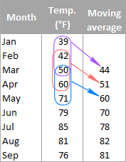
Generally speaking, moving average (also referred to as rolling average, running average or moving mean) can be defined as a series of averages for different subsets of the same data set.
It is frequently used in statistics, seasonally-adjusted economic and weather forecasting to understand underlying trends. In stock trading, moving average is an indicator that shows the average value of a security over a given period of time. In business, it's a common practice to calculate a moving average of sales for the last 3 months to determine the recent trend.
For example, the moving average of three-month temperatures can be calculated by taking the average of temperatures from January to March, then the average of temperatures from February to April, then of March to May, and so on.
There exist different types of moving average such as simple (also known as arithmetic), exponential, variable, triangular, and weighted. In this tutorial, we will be looking into the most commonly used simple moving average.
Calculating simple moving average in Excel
Overall, there are two ways to get a simple moving average in Excel - by using formulas and trendline options. The following examples demonstrate both techniques.
Calculate moving average for a certain time period
A simple moving average can be calculated in no time with the AVERAGE function. Supposing you have a list of average monthly temperatures in column B, and you want to find a moving average for 3 months (as shown in the image above).
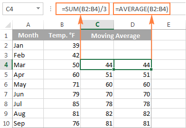
Write a usual AVERAGE formula for the first 3 values and input it in the row corresponding to the 3rd value from the top (cell C4 in this example), and then copy the formula down to other cells in the column:
=AVERAGE(B2:B4)
You can fix the column with an absolute reference (like $B2) if you want to, but be sure to use relative row references (without the $ sign) so that the formula adjusts properly for other cells.
Remembering that an average is computed by adding up values and then dividing the sum by the number of values to be averaged, you can verify the result by using the SUM formula:
=SUM(B2:B4)/3
Get moving average for a the last N days / weeks / months/ years in a column
Supposing you have a list of data, e.g. sale figures or stock quotes, and you want to know the average of the last 3 months at any point of time. For this, you need a formula that will recalculate the average as soon as you enter a value for the next month. What Excel function is capable of doing this? The good old AVERAGE in combination with OFFSET and COUNT.
Where N is the number of the last days / weeks / months/ years to include in the average.
Not sure how to use this moving average formula in your Excel worksheets? The following example will make things clearer.
Assuming that the values to average are in column B beginning in row 2, the formula would be as follows:
=AVERAGE(OFFSET(B2,COUNT(B2:B100)-3,0,3,1))
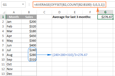
And now, let's try to understand what this Excel moving average formula is actually doing.
- The COUNT function COUNT(B2:B100) counts how many values are already entered in column B. We start counting in B2 because row 1 is the column header.
- The OFFSET function takes cell B2 (the 1st argument) as the starting point, and offsets the count (the value returned by the COUNT function) by moving 3 rows up (-3 in the 2nd argument). As the result, it returns the sum of values in a range consisting of 3 rows (3 in the 4th argument) and 1 column (1 in the last argument), which is the latest 3 months that we want.
- Finally, the returned sum is passed to the AVERAGE function to calculate the moving average.
Tip. If you are working with continuously updatable worksheets where new rows are likely to be added in the future, be sure to supply a sufficient number of rows to the COUNT function to accommodate potential new entries. It's not a problem if you include more rows than actually needed as long as you have the first cell right, the COUNT function will discard all empty rows anyway.
As you probably noticed, the table in this example contains data for only 12 months, and yet the range B2:B100 is supplied to COUNT, just to be on the save side :)
Find moving average for the last N values in a row
If you want to calculate a moving average for the last N days, months, years, etc. in the same row, you can adjust the Offset formula in this way:
Supposing B2 is the first number in the row, and you want to include the last 3 numbers in the average, the formula takes the following shape:
=AVERAGE(OFFSET(B2,0,COUNT(B2:N2)-3,1,3))

Creating an Excel moving average chart
If you have already created a chart for your data, adding a moving average trendline for that chart is a matter of seconds. For this, we are going to use Excel Trendline feature and the detailed steps follow below.
For this example, I've created a 2-D column chart (Insert tab > Charts group) for our sales data:
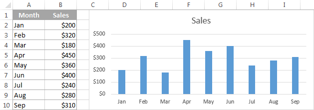
And now, we want to "visualize" the moving average for 3 months.
- In Excel 2013, select the chart, go to the Design tab > Chart Layouts group, and click Add Chart Element > Trendline > More Trendline Options…

In Excel 2010 and Excel 2007, go to Layout > Trendline > More Trendline Options.
Tip. If you do not need to specify the details such as the moving average interval or names, you can click Design > Add Chart Element > Trendline > Moving Average for the immediate result.
- The Format Trendline pane will open on the right-hand side of your worksheet in Excel 2013, and the corresponding dialog box will pop up in Excel 2010 and 2007.
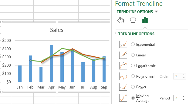
On the Format Trendline pane, you click the Trendline Options icon, select the Moving Average option and specify the moving average interval in the Period box:

- Close the Trendline pane and you will find the moving average trendline added to your chart:
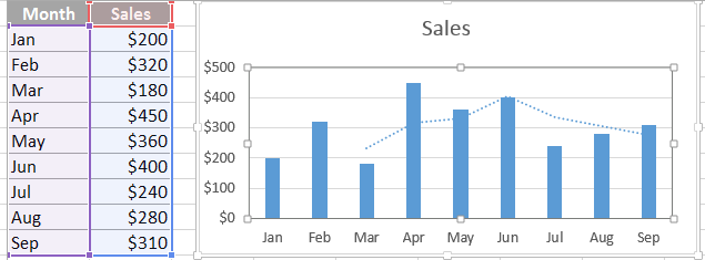
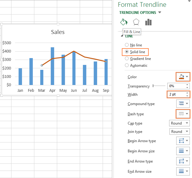
To refine your chat, you can switch to the Fill & Line or Effects tab on the Format Trendline pane and play with different options such as line type, color, width, etc.
For powerful data analysis, you may want to add a few moving average trendlines with different time intervals to see how the trend evolves. The following screenshot shows the 2-month (green) and 3-month (brick red) moving average trendlines:
Well, that's all about calculating moving average in Excel. The sample worksheet with the moving average formulas and trendline is available for download at the end of this post. I thank you for reading and look forward to seeing you next week!
Practice workbook
Calculating moving average - examples (.xlsx file)
 by
by
28 comments
Hi Alex,
How would I go about this in the reverse? Ie; What I need my average sale to be to reach my budget?
As an example; my budget is 20,000. I have gotten 15 sales so far in the year for 8,000 total, and expecting another 15 sales for the rest of the year. I would need an average of 800 per sale to reach my budget.
But how do I put this in a formula so it will show the average sale required to reach my budget (or goal in this case)?
Thank you :)
This is a task for the school: (20000-8000)/15
Can we do this same when performing weighted moving average? If yes, how to go about it. Thanks.
Hi! Maybe this article will be helpful: How to calculate weighted average in Excel.
This is in reference to: "Find moving average for the last N values in a row"
How would the formula change if you are trying to find the MA for the FIRST N values instead of the last? I have my data set up in reverse chronological order for a scorecard.
Thanks!
I tried a different approach. Went to the "Define Name" part of the Formulas tab and named cells F6:R6 as "Rolling_Average" and then I entered =Average(Rolling_Average) in cell E6. The Rolling average forumla seems to average F6:R6 regardless of how many columns I add.
Hi
Super tutorial. Thanks.
Can anyone help with this?
I'm trying 7 day rolling average for an entire column (A:A) which gets added to everyday (blanks at the end of column ignored) and output that result to an assigned cell. That's explained perfectly in the tutorial above.
But how do I calculate rolling average for entire column entries except the last entry and this result returned to another assigned cell?
I.E - if I have 100 days data in a column. I want rolling average from days 94-100 returned to a particular cell. I also want rolling average for days 93-99 returned to another cell and rolling average for days 92-98 returned to a 3rd cell?
Thanks
D
Hi!
With the OFFSET function, you can get the range of values you need.
=OFFSET(B1,COUNT(B1:B100)-8,0,7,1)
=OFFSET(B1,COUNT(B1:B100)-9,0,7,1)
=AVERAGE( OFFSET(B1,COUNT(B1:B100)-9,0,7,1) )
This should solve your task.
what is the formula to average a column (in the adjacent column) each time a new (entry) row is added at the bottom? in other words, the first cell of the average is always the top cell in the original column, but the last cell to be included in the average is the new row.
Hello!
If I understand you correctly, you want to calculate the average in one cell. The AVERAGE function ignores empty cells. Therefore, you can calculate the average over a large data range to which you will add new data.
For example, = AVERAGE (F2: F1000)
If my guess is not correct, then use the instruction from Example 1 above.
I have a spreadsheet of distance travelled on my bike working towards a target distance with a month. I would like to create a formula showing me how many miles per day i need to average to achieve the distance but one that adjusts to the days remaining in the month as i don't work out every day.
Hello!
I do not know how your data is written. But I think this formula will be useful to you.
=(B1-SUM(A2:A31))/(EOMONTH(TODAY(),0)-TODAY())
A2:A31 - daily miles data. B1 - target distance for a month.
I'm tracking numbers for a Skeet League. Calculating moving average for their last 20 scores. The names entered down (each person has their own row), and scores recorded daily in columns. Sometimes people are absent, so we leave that blank for that person on that date. So moving average gives us an incorrect number, because it uses the "0" value????
Hello, Guy,
To include a condition to your formula (">0"), try using AVERAGEIF instead. You will find formula examples in this article.
Hi Svetlana,
First of all thanks for this helpful article. I need one info, can we show value of average point in graph. Please let me know.
Thanks,
Kiran
Hello Kiran,
The second part of this tutorial shows how to display the moving average in a graph by using the Trendline Options. If you are looking for something different, please clarify.
Please help with the correct formula to calculate the sum of hours entered on a moving 7 day period. For example. I need to know how much overtime is worked by an individual over a rolling 7 day period calculated from the beginning of the year to the end of the year. The total amount of hrs worked must update for the 7 rolling days as I enter the overtime hours in on a daily basis
Thank you
I am looking for something very similar! I am looking for the last 6 months! I'm so stumped!
Your example 3 above (Get moving average for the last N values in a row) worked perfectly for me if the whole row contains numbers. I'm doing this for my golf league where we use a 4 week rolling average. Sometimes the golfers are absent so instead of a score, I will put "ABS" (text) in the cell. I still want the formula to look for the last 4 scores and not count the "ABS" either in the numerator or in the denominator. How do I modify the formula to accomplish this?
Yes, I did notice if cells were empty the calculations were incorrect. In my situation I am tracking over 52 weeks. Even if the last 52 weeks contained data, the calculation was incorrect if any cell prior to the 52 weeks was blank.
Hi .. I really liked the way it has been explained and was able to do in in a minute.. I also liked your website and will follow it regularly..
I was working with a e excel file where i required to make a moving average of last 2 months data which were in different column i.e(D3:G2)
Can you please let me know what modification is required in the formula so that i can make it work to calculate the same..
Rishabh
Hi Rishabh,
Thank you for your feedback. Assuming that you need a moving average for the last 2 numbers in the same row, you can adjust the formula in this way:
=AVERAGE(OFFSET(D3, 0, COUNT(D3:Z3)-2,1,2))
Where D3 is the first number in the row, and 2 is the number of the last N months to be included in the average.
Hi,
I have 1000 numbers starting from 1 to 1000. i want average for every 3 numbers. say from 1 to 3 it should be 2. now my next number will be 4 to 6 then 7 to 10 and so on up to 1000 numbers.
If i use average function then it will do average for 1 to 3 then 2 to 4 then 3 to 5. it is not meeting my requirement.
please help me to solve this case.
Hi nikhil,
I can help you in this...you have to use indirect function to achieve this task
You can use average (indirect ("b"&rows (b$1$:b1)*3-2&":"&"b"&rows(b $1$:b1)*3))
To calculate average for column b for every 3 sets of numbers
✌
Hi,
I need your help on this please. I have "column A" with dates and "column B" with values which has both negative and positive values in it. i want to calculate "average" for a particular date from "columb B". Can you please help me on how to calculate average only for the positive values from "column B".
Thank you for your help in advance.
Hello, Yogi,
Please try one of these formulas:
=AVERAGEIF(B:B,"= 42386",A:A) or
=AVERAGEIF(B:B,B3,A:A)
In these formulas please replace 42386 or B3 with the needed parameter.
Hi,
I have read through several different articles looking for an answer to my problem, got lots of great tips but nothing defiant that helps me now.
Could you please help me on this? I’m trying to create a formula that adds the total amount for a particular supplier that is more than 30 days & in another cell a formula that is more than 60 days, etc…
I have the dates of invoices in column A, supplier’s names in column B and Total value in column C.
Any help would be appreciated, have spent days on this & to no avail. Thanks
Hi Kay,
I think you can use the SUMIFS function. For example, to find the total for supplier "John" for orders made more than 30 days ago, you can use the following formula:
=SUMIFS(C2:C100, B2:B100, "john", A2:A100,"<"&TODAY()-30)
For the detailed explanation of SUMIFS' arguments and more formula examples, please see How to use Excel SUMIFS and SUMIF with multiple criteria.