While Microsoft Excel provides an array of functions to work with weekdays, months and years, only one is available for weeks - the WEEKNUM function. So, if you are looking for a way to get a week number from a date, WEEKNUM is the function you want.
In this short tutorial, we will briefly talk about the syntax and arguments of Excel WEEKNUM, and then discuss a few formula examples demonstrating how you can use the WEEKNUM function to calculate week numbers in your Excel worksheets.
Excel WEEKNUM function - syntax
The WEEKNUM function is used in Excel to return the week number of a specific date in the year (a number between 1 and 54). It has two arguments, the 1st is required and the 2nd is optional:
- Serial_number - any date within the week whose number you are trying to find. This can be a reference to a cell containing the date, a date entered by using the DATE function or returned by some other formula.
- Return_type (optional) - a number that determines on which day the week begins. If omitted, the default type 1 is used (the week beginning on Sunday).
Here is a complete list of the return_type values supported in WEEKNUM formulas.
| Return_type | Week begins on |
| 1 or 17 or omitted | Sunday |
| 2 or 11 | Monday |
| 12 | Tuesday |
| 13 | Wednesday |
| 14 | Thursday |
| 15 | Friday |
| 16 | Saturday |
| 21 | Monday (used in System 2, please see the details below.) |
In the WEEKNUM function, two different week numbering systems are used:
- System 1. The week containing January 1 is considered the 1st week of the year and is numbered week 1. In this system, the week traditionally starts on Sunday.
- System 2. This is the ISO week date system that is part of the ISO 8601 date and time standard. In this system, the week starts on Monday and the week containing the first Thursday of the year is considered week 1. It is commonly known as the European week numbering system and it is used mainly in government and business for fiscal years and timekeeping.
All of the return types listed above apply to System 1, except for return type 21 that is used in System 2.
Note. In Excel 2007 and earlier versions, only options 1 and 2 are available. Return types 11 through 21 are supported in Excel 2010 and Excel 2013 only.
Excel WEEKNUM formulas to convert date to week number (from 1 to 54)
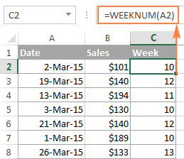
The following screenshot demonstrates how you can get week numbers from dates with the simplest =WEEKNUM(A2) formula:

In the above formula, the return_type argument is omitted, which means that the default type 1 is used - the week beginning on Sunday.
If you'd rather begin with some other day of the week, say Monday, then use 2 in the second argument:
=WEEKNUM(A2, 2)
Instead of referring to a cell, you can specify the date directly in the formula by using the DATE(year, month, day) function, for example:
=WEEKNUM(DATE(2015,4,15), 2)
The above formula returns 16, which is the number of the week containing April 15, 2015, with a week beginning on Monday.
In real-life scenarios, the Excel WEEKNUM function is rarely used on its own. Most often you would use it in combination with other functions to perform various calculations based on the week number, as demonstrated in further examples.
How to convert week number to date in Excel
As you have just seen, it's no big deal to turn a date into a week number using the Excel WEEKNUM function. But what if you are looking for the opposite, i.e. converting a week number to a date? Alas, there is no Excel function that could do this straight away. So, we will have to construct our own formulas.
Supposing you have a year in cell A2 and a week number in B2, and now you want to calculate the Start and End dates in this week.

Note. This formula example is based on ISO week numbers, with a week starting on Monday.
The formula to return the Start date of the week is as follows:
=DATE(A2, 1, -2) - WEEKDAY(DATE(A2, 1, 3)) + B2 * 7
Where A2 is the year and B2 is the week number.
Please note that the formula returns the date as a serial number, and to have it displayed as a date, you need to format the cell accordingly. You can find the detailed instructions in Changing date format in Excel. And here is the result returned by the formula:

Of course, the formula to convert a week number to a date is not trivial, and it may take a while to get your head round the logic. Anyway, I will do my best to provide meaningful explanation for those who are curious to get down to the bottom.
As you see, our formula consists of 2 parts:
DATE(A2, 1, -2) - WEEKDAY(DATE(A2, 1, 3))- calculates the date of the last Monday in the previous year.B2 * 7- adds the number of weeks multiplied by 7 (the number of days in a week) to get the Monday (start date) of the week in question.
In the ISO week numbering system, week 1 is the week containing the first Thursday of the year. Consequently, the first Monday is always between December 29 and January 4. So, to find that date, we have to find the Monday immediately before January 5.
In Microsoft Excel, you can extract a day of week from a date by using the WEEKDAY function. And you can use the following generic formula to get Monday immediately before any given date:
If our ultimate goal were to find Monday immediately before the 5th of January of the year in A2, we could use the following DATE functions:
=DATE(A2,1,5) - WEEKDAY(DATE(A2,1,3))
But what we actually need is not the first Monday of this year, but rather the last Monday of the previous year. So, you have to subtract 7 days from January 5 and hence you get -2 in the first DATE function:
=DATE(A2,1,-2) - WEEKDAY(DATE(A2,1,3))
Compared to the tricky formula you have just learned, calculating the End date of the week is a piece of cake :) To get Sunday of the week in question, you simply add 6 days to the Start date, i.e. =D2+6

Alternatively, you could add 6 directly in the formula:
=DATE(A2, 1, -2) - WEEKDAY(DATE(A2, 1, 3)) + B2 * 7 + 6
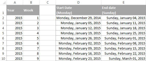
To make sure the formulas always deliver the right dates, please have a look at the following screenshot. The Start Date and End Date formulas discussed above are copied across column D and E, respectively:
Other ways to convert week number to date in Excel
If the above formula based on the ISO week date system does not meet your requirements, try one of the following solutions.
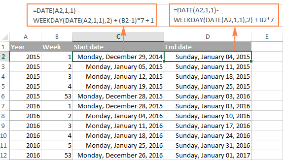
Formula 1. A week containing Jan-1 is week 1, Mon-Sun week
As you remember, the previous formula works based on the ISO date system where the first Thursday of the year is considered week 1. If you work based on a date system where the week containing the 1st of January is considered week 1, use the following formulas:
Start date:
=DATE(A2,1,1) - WEEKDAY(DATE(A2,1,1),2) + (B2-1)*7 + 1
End date:
=DATE(A2,1,1)- WEEKDAY(DATE(A2,1,1),2) + B2*7
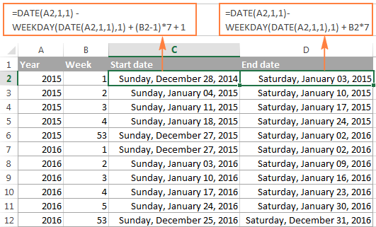
Formula 2. A week containing Jan-1 is week 1, Sun-Sat week
These formulas are similar to the above ones with the only difference that they are written for Sunday - Saturday week.
Start date:
=DATE(A2,1,1) - WEEKDAY(DATE(A2,1,1),1) + (B2-1)*7 + 1
End date:
=DATE(A2,1,1)- WEEKDAY(DATE(A2,1,1),1) + B2*7
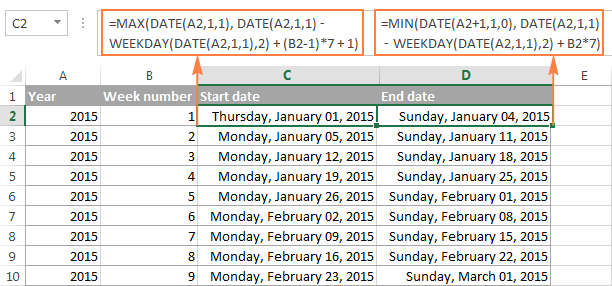
Formula 3. Always start counting on January 1, Mon-Sun week
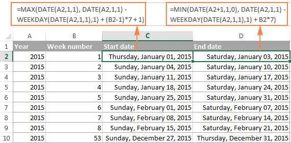
While the previous formulas return Monday (or Sunday) of week 1, regardless of whether if falls within this year or the previous year, this start date formula always returns January 1 as the start date of week 1 regardless of the day of the week. By analogy, the end date formula always returns December 31 as the end date of the last week in the year, regardless of the day of the week. In all other respects, these formulas work similarly to Formula 1 above.
Start date:
=MAX(DATE(A2,1,1), DATE(A2,1,1) - WEEKDAY(DATE(A2,1,1),2) + (B2-1)*7 + 1)
End date:
=MIN(DATE(A2+1,1,0), DATE(A2,1,1) - WEEKDAY(DATE(A2,1,1),2) + B2*7)
Formula 4. Always start counting on January 1, Sun-Sat week
To calculate the start and end dates for a Sunday - Saturday week, all it takes is one small adjustment in the above formulas :)
Start date:
=MAX(DATE(A2,1,1), DATE(A2,1,1) - WEEKDAY(DATE(A2,1,1),1) + (B2-1)*7 + 1)
End date:
=MIN(DATE(A2+1,1,0), DATE(A2,1,1) - WEEKDAY(DATE(A2,1,1),1) + B2*7)
How to get month from week number
To get a month corresponding to the week number, you find the first day in a given week as explained in this example, and then wrap that formula in the Excel MONTH function like this:
=MONTH(DATE(A2, 1, -2) - WEEKDAY(DATE(A2, 1, 3)) + B2 * 7)
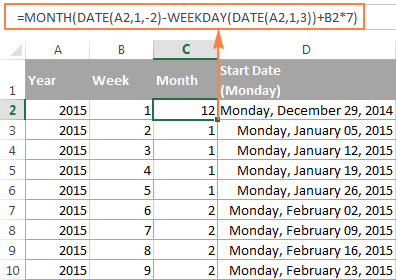
Note. Please remember that the above formula works based on the ISO week date system, where the week starts on Monday and the week containing the 1st Thursday of the year is considered week 1. For example, in the year 2016, the first Thursday is January 7, and that is why week 1 begins on 4-Jan-2016.
How to get a week number in a month (from 1 to 6)
If your business logic requires converting a specific date to the week number within the corresponding month, you can use the combination of WEEKNUM, DATE and MONTH functions:
Assuming that cell A2 contains the original date, use the following formula for a week beginning on Monday (notice 21 in WEEKNUM's return_type argument):
=WEEKNUM($A2,21)-WEEKNUM(DATE(YEAR($A2), MONTH($A2),1),21)+1
For a week beginning on Sunday, omit the return_type argument:
=WEEKNUM($A2)-WEEKNUM(DATE(YEAR($A2), MONTH($A2),1))+1

How to sum values and find average by the week number
Now that you know how to convert a date to a week number in Excel, let's see how you can use week numbers in other calculations.
Suppose, you have some monthly sales figures and you want to know the total for each week.
To begin with, let's find out a week number corresponding to each sale. If your dates are in column A and sales in column B, copy the =WEEKNUM(A2) formula across column C beginning in cell C2.
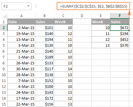
And then, make a list of week numbers in some other column (say, in column E) and calculate the sales for each week using the following SUMIF formula:
=SUMIF($C$2:$C$15, $E2, $B$2:$B$15)
Where E2 is the week number.
In this example, we are working with a list of March sales, so we have week numbers 10 to 14, as demonstrated in the following screenshot:
In a similar manner, you can calculate the sales average for a given week:
=AVERAGEIF($C$2:$C$15, $E2, $B$2:$B$15)
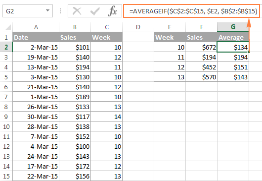
If the helper column with the WEEKNUM formula does not fit well into your data layout, I regret to tell you that there is no simple way to get rid of it because Excel WEEKNUM is one of those functions that doesn't accept range arguments. Therefore, it cannot be used within SUMPRODUCT or any other array formula like the MONTH function in a similar scenario.
How to highlight cells based on the week number
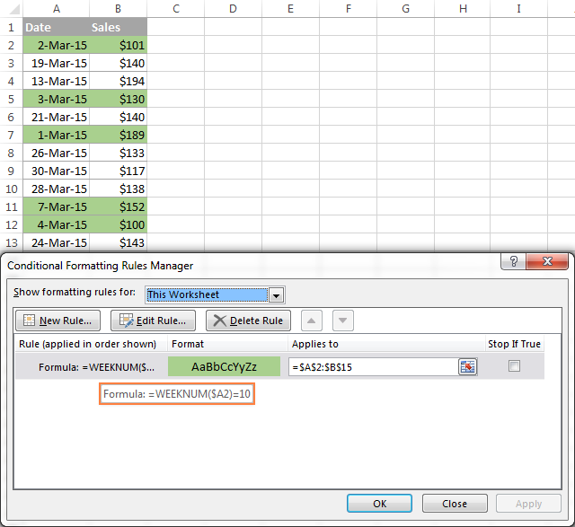
Let's say you have a long list of dates in some column and you want to highlight only those that relate to a given week. All you need is a conditional formatting rule with a WEEKNUM formula similar to this:
=WEEKNUM($A2)=10
As demonstrated in the screenshot below, the rule highlights sales that were made within week 10, which is the first week in March 2015. Since the rule applies to A2:B15, it highlights values in both columns. You can learn more about creating conditional formatting rules in this tutorial: Excel conditional formatting based on another cell value.
This is how you can calculate week numbers in Excel, convert week number to date and extract week number from date. Hopefully, the WEEKNUM formulas you have learned today will prove useful in your worksheets. In the next tutorial, we will talk about calculating age and years in Excel. I thank you for reading and hope to see you next week!
 by
by
80 comments
Dear Alexander;
Regarding "How to convert week number to date in Excel"
The formula =DATE(A2, 1, -2) - WEEKDAY(DATE(A2, 1, 3)) + B2 * 7 is fantastic, and does work, but ...
Can you explain the use of 3 in the section WEEKDAY(DATE(A2, 1, 3)) !
In other words: "Why subtract the result of the third day of the first month in any given year?
Why 3 and not 1?
Hello Mark!
The first Monday is always December 29th to January 4th. Therefore, we subtract the number of the weekday of 3 January in order to get the date of the last Monday of the previous year.
Week Description Act BUD
August Week1 45 55
August Week2 16 55
August Week3 55
August Week4 32 55
August Week5 55
Kind assistance, is there are way I can get an August Week4 YTD BUD value of 220 in a cell, at the end of that week the corresponding YTD Act will be (45+16+0+32=93).
Thanking in advance.
HC
Hi! If I understand your task correctly, this article may be helpful: Excel Cumulative Sum - easy way to calculate running total.
Suppose your data are in column C, please try to enter the following formula in cell E2 and then copy it down along the column:
=SUM($C$2:C2)
I see above you answer how to change week number for when week 1 starts in April. I have tried to use that formula and change some of it to allow me to use it for what I require but cannot find the problem causing #VALUE error. I need week 1 to start the 1st Monday of December 23 and count the 52 weeks up from there, unsure if it is because it starts in a different year it is the problem?
Any help would be appreciated.
Hi! If I understand your task correctly, try the following formula:
=ROUNDDOWN((A1-$G$1)/7+1,0)
$G$1 - is the date on which the week numbers begin.
For sorting purpose, how do you ge the "0" in front of weeks 1-9? Example WEEK1 to look like WEEK01?
Hi! If I understand your task correctly, this guide may be helpful: How to add leading zeros in Excel. You can add zeros before a number using the TEXT function and other methods described in this article. For example:
="Week"&TEXT(WEEKNUM(A1),"00")
Hello! I have all data in this format: i.e
Input: 2401.5 which means = year 2024, week 1, day 5.
How can I translate this into 05/January/2024 ?
Thank you
Hi! Use substring functions LEFT, Right and MID to extract text strings. Use the DATE function to set the date to January 1, then add the desired number of days.
For more information, please visit: Excel substring functions to extract text from cell.
=DATE("20"&LEFT(A1,2),1,1)+(MID(A1,3,2)-1)*7+RIGHT(A1,1)-1
Good Afternoon ALCON,
I have three date related formulas where, if there is no data in the corresponding field, there is still a return value. Case in point: =WEEKNUM([@[Check-Out Date]],1)-40+IF(MONTH([@[Check-Out Date]])<10,53,1) will return with "13" if the "Check-Out Date" field is blank. Is there a way to adjust the formula to have the field remain blank? The other formulas in question are: =MONTH([@[Check-Out Date]])-10+IF(MONTH([@[Check-Out Date]])<10,13,1) which returns "4" and = YEAR([@[Check-Out Date]]) which returns "1900"
Hi! I can't check and correct a formula that contains unique references to your data. To perform calculations only when a date is written in the cell, add a condition using the IF function.
For example,
IF(A1<>"", [formula],"")
Read more: IF function in Excel: formula examples for text, numbers, dates, blanks.
I have Date and month in excel data. I want to get week number which 1st monday included in that month. How to get that?
Hi! To find the date of the first Monday of the month, use the formula:
=DATE(YEAR(D1),MONTH(D1),(D3*7)+1) - WEEKDAY(DATE(YEAR(D1),MONTH(D1),8-D2),2)
D1 - any date of the month
D2 - number for the week (starting with Monday)
D3 - Nth occurrence in the month
To find the week number, add the WEEKNUM function.
=WEEKNUM(DATE(YEAR(D1),MONTH(D1),(D3*7)+1) - WEEKDAY(DATE(YEAR(D1),MONTH(D1),8-D2),2))
sir .
excel 2007 does not many return_type please explain how i should start Friday to Thursday ?
Hi! Set return_type to 15. Read first paragraph of this article.
Hello all experts,
I have a task which needs to return every first and third Wednesday of each month and every second and fourth Monday of each month.
The tricky part is, we don't use the ISO week system. We simply use the first week of that month. Meaning that for example Feb 2023, 1/2/2023 is Wednesday, and this is the first week. So no first Monday will be return on that month and the second Monday should return 6 Feb 2023 and fourth Monday will be 20 Feb 2023 and so on using the same algorithm for every month and every year.
Is there any way by using formula to achieve this, please advise.
Thank you so much in advance.
Can anyone please help?
Dear All,
I have a question. I have to make an excel function. A have a column with Year (in format 2021.01.01), a Week Nr. (in format 1-52). I have to make a third column for the following method:
Concatenating the year (from a column containg the year in format 2012.01.01),
a letter "W" and the Week Nr (a Week Nr smaller than 10 must be preceded by a "0", e.g. 2012W01).
--A made the calculation for the Week Nr (with the WEEKNUM function, the second parameter of which is: 21 (this is the ISO 8601 week number, the
week containing the first Thursday of the year is week 1)).
-- It is interesting, that the Week nr of 2012.12.31 was/is 1 week. Is it an error, or I have to make a calculation, to not repeat it (because theree is 1st
week in 2012.01.01-2012.01.8?
Please help me. Thank you.
Hi!
Try using parameter 2 in the WEEKNUM function.
How can I create a work schedule with following : 4days off , 5days on , 4 days off , 5 days on, 5days off , 4 days on , 5 days off,
For a year , the working is like that .
Ex : starting on 1 January 2023
Thank you
Hi!
I don't see any pattern in your data. If there is, please describe.
Hi,
How can I convert my work week number to date or vice versa.
Example:
1) Input = 25.3, Output = 15/06/2022
2) Input = 15/06/2022 to WW25.3
here the week number starting from Monday.
Hello!
To convert a week number to a date, try this formula with WEEKDAY function:
=MAX(DATE(YEAR(TODAY()),1,1),DATE(YEAR(TODAY()),1,1) - WEEKDAY(DATE(YEAR(TODAY()),1,1),2) + (A2-1)*7+1)
Thank you so much, That's perfectly working.
Can you also tell us how to do in reverse.
I mean if I enter date it should give me work week number.
Example:
Input = 15/06/2022 then it should give the output as WW25.3
Thanks in advance...
Hi!
To get the number after the decimal point, use the WEEKDAY function.
=WEEKNUM(D1) + WEEKDAY(D1,2)/10
Please how can I calculate week 38 to months
Hello!
To determine the month number, use the MONTH function
Please try the following formula:
=MONTH(A1*7)
or
=MONTH(A1*7+DATE(YEAR(TODAY()),1,1))
Here the month number is calculated from the last day of the week.
Hi,
Is there a way to convert a week number (i.e 19) to a date format (1/23/2022) given current date?
Thank you so much!
Hello!
The answer to your question is in this manual: How to convert week number to date.
I hope my advice will help you solve your task.
Thank you, I appreciate your help!
Hi!
Any ideas whether to use an ISOWEEKNUM function or a Format Cells option:
e.g. a project starts in week X, no binding to date or year.
Different activities are to be accomplished prior to the project start - let's say task A: week "X- 7" before project start, task B: week "X - 4" before, task C: week "X - 2" before, etc..
How can a project start week be determined as a week nr for excel, otherwise week 3 starting project shows "-4" for task A instead of 49.
Thanks,
Daniel
Hi!
The week number can only be determined by the date. You have no date.
Hi,
My financial year starts from 1st April and whatever day it is it should be week 1 and should change to next week after Sunday. Means week is calculated from Monday to Sunday.
1st April'20 to 5 April - week1
6th April to 12 April - week 2
And further proceed in similar way till 31st March'21.
Pls suggest the formula.
TIA
Hello!
I believe the following formula will help you solve your task:
=IF(MONTH(A2)>3,WEEKNUM(A2,2)-13,WEEKNUM(DATE(YEAR(A2),12,31),2)+WEEKNUM(A2)-13)
Wonderful answer Alexander...
Please try to decrease the length of formula so beginners can understand easily. The below is example for Jul-Jun financial year.
=IF(MONTH(A2)>6,WEEKNUM(A2,2)-27,53+WEEKNUM(A2)-27)
Hello!
I have a scenario where we want to take the date and convert that date to say 'week of Sep 20th" which would be the Monday of that week
my date is 23-SEP-2021 - i can use "=A2-WEEKDAY(A2,2)+1" to get the Monday date
result: 20-SEP-2021
But can it be converted all at once to return "Week of Sep 20th" instead using the original date of Sep 23?
Hello!
If I understand your task correctly, the following formula should work for you:
=CONCATENATE("Week of ",TEXT(A2-WEEKDAY(A2,2)+1,"mmm")," ", DAY(A2-WEEKDAY(A2,2)+1) & LOOKUP(DAY(A2-WEEKDAY(A2,2)+1), {1,"st";2,"nd";3,"rd";4,"th";21,"st";22,"nd";23,"rd";24,"th";31,"st"}))
Hello,
Could you please solve my issue. I have cell criteria, A1 = year, B1 = month and C1 = week number. My week starts on Sunday. 1 to 4 March 2021 should be the first week and 6 to 11 March 2021 should be the second week. If I change the cell value C1 = 6 than formula return should be blank. Hence, it should not bring any date from any other month.
DATE(A1,MONTH(B1),1) - WEEKDAY(DATE(A1,MONTH(B1),1),1)+ (C1-1)*7
Sorry ,Just small correction, My week starts on Saturday
Thank you. I was looking for this.
I use Excel 2010 so I had to convert all the ; and also it's a Danish version So I had to change the Max to Maks, Date to Dato, and weekday to Ugedag. Then it worked brilliantly ☺
I made a typo ☺.
I had to change all the , commas to ; semicolon for it work in Excel 2010
Is there a way to use =WEEKNUM(TODAY()), but have it display in the cell with additional text before and after, i want the text to stay the same, but i want the Week Number to auto update each time someone opens the spreadsheet
Week 47 Thu
Hello!
Please check out this article to learn how to combine text with a formula-driven value.
If there is anything else I can help you with, please let me know.