This tutorial shows how to sum a column in Excel 2010 - 2016. Try out 5 different ways to total columns: find the sum of the selected cells on the Status bar, use AutoSum in Excel to sum all or only filtered cells, employ the SUM function or convert your range to Table for easy calculations.
If you store such data as price lists or expense sheets in Excel, you may need a quick way to sum up prices or amounts. Today I'll show you how to easily total columns in Excel. In this article, you'll find tips that work for summing up the entire column as well as hints allowing to sum only filtered cells in Excel.
Below you can see 5 different suggestions showing how to sum a column in Excel. You can do this with the help of the Excel SUM and AutoSum options, you can use Subtotal or turn your range of cells into Excel Table which will open new ways of processing your data.
How to sum a column in Excel with one click
There is one really fast option. Just click on the letter of the column with the numbers you want to sum and look at the Excel Status bar to see the total of the selected cells.
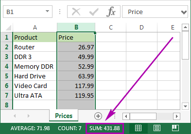
Being really quick, this method neither allows copying nor displays numeric digits.
How to total columns in Excel with AutoSum
If you want to sum up a column in Excel and keep the result in your table, you can employ the AutoSum function. It will automatically add up the numbers and will show the total in the cell you select.
- To avoid any additional actions like range selection, click on the first empty cell below the column you need to sum.
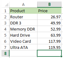
- Navigate to the Home tab -> Editing group and click on the AutoSum button.

- You will see Excel automatically add the =SUM function and pick the range with your numbers.
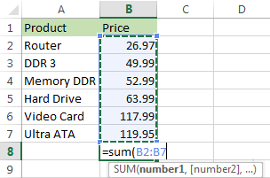
- Just press Enter on your keyboard to see the column totaled in Excel.
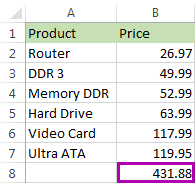
This method is fast and lets you automatically get and keep the summing result in your table.
Use the SUM function to total a column
You can also enter the SUM function manually. Why would you need this? To total only some of the cells in a column or to specify an address for a large range instead of selecting it manually.
- Click on the cell in your table where you want to see the total of the selected cells.

- Enter
=sum(to this selected cell.
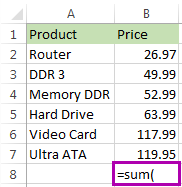
- Now select the range with the numbers you want to total and press Enter on your keyboard.
Tip. You can enter the range address manually like
=sum(B1:B2000). It's helpful if you have large ranges for calculation.

That's it! You will see the column summed. The total will appear in the correct cell.

This option is really handy if you have a large column to sum in Excel and don't want to highlight the range. However, you still need to enter the function manually. In addition, please be prepared that the SUM function will work even with the values from hidden and filtered rows. If you want to sum visible cells only, read on and learn how.
Tips:
- Using the SUM function, you can also automatically total new values in a column as they are added and calculate the cumulative sum.
- To multiply one column by another, use the PRODUCT function or multiplication operator. For full details, please see How to multiply two or more columns in Excel.
Use Subtotal in Excel to sum only filtered cells
This feature is perfect for totaling only the visible cells. As a rule, these are filtered or hidden cells.
- First, filter your table. Click on any cell within your data, go to the Data tab and click on the Filter icon.

- You will see arrows appear in the column headers. Click on the arrow next to the correct header to narrow down the data.
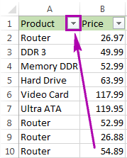
- Uncheck Select All and tick off only the value(s) to filter by. Click OK to see the results.

- Select the range with the numbers to add up and click AutoSum under the Home tab.
 Voila! Only the filtered cells in the column are summed up.
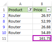
If you want to sum visible cells but don't need the total to be pasted to your table, you can select the range and see the sum of the selected cells on the Excel Status bar. Or you can go ahead and see one more option for summing only filtered cells.
Convert your data into Excel table to get total for your column
If you often need to sum columns, you can convert your spreadsheet to Excel Table. This will simplify totaling columns and rows as well as performing many other operations with your list.
- Press Ctrl + T on yourkeyboardto format the range of cells as Excel Table.
- You will see the new Design tab appear. Navigate to this tab and tick the checkbox Total Row.

- A new row will be added at the end of your table. To make sure you get the sum, select the number in the new row and click on the small down arrow next to it. Pick the Sum option from the list.
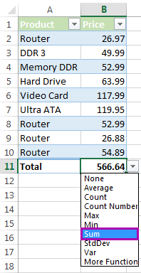 Using this option lets you easily display totals for each column. You can see sum as well as many other functions like Average, Min and Max.
This feature adds up only visible (filtered) cells. If you need to calculate all data, feel free to employ instructions from How to total columns in Excel with AutoSum and Enter the SUM function manually to total the column.
Whether you need to sum the entire column in Excel or total only visible cells, in this article I covered all possible solutions. Choose an option that will work for your table: check the sum on the Excel Status bar, use the SUM or SUBTOTAL function, check out the AutoSum functionality or format your data as Table.
If you have any questions or difficulties, don't hesitate to leave comments. Be happy and excel in Excel!
 by
by
55 comments
I have an excel sheet with data in rows, with the periodic billing order number in column A, customer ID in column B, and the approved amount in Column C. There might be only 5 rows of data for a particular customer ID or there might be twelve. I need to create a list which includes the total approved order amounts from column C for each customer ID in column B.
Hi! If you want to find the sum of approved orders for each customer, try using the SUMIFS function. The following tutorial should help: How to use Excel SUMIFS and SUMIF with multiple criteria. I hope it’ll be helpful. If this is not what you wanted, please describe the problem in more detail.
how about sum total formula from formula numbers how can i total, it cant be read if i used sum of..
thanks for the answer.
Hi!
What do you want to calculate exactly? Your question is not completely clear, please specify.
Hi Ryan,
Thank you so much for a very helpful post. I am creating a timesheet template but the total for the hours worked is incorrect. On the particular cell, I used the formula: =SUM(G5:G11), and it should give the total number of hours worked in a week. Not sure what I am not doing right, the data entries are in the form: hhmmss.
Hello!
I think an article on how you can perform mathematical operations with time will be useful to you: Calculate time in Excel- time difference, add, subtract and sum times.
Is there a way to sum a column where every cell is the sum of 2 different cells? Every time I try it adds the formulas together and I end up with my original number.
Ie
C3 =b2-b3
C4 =b3-b4
C5 =b4-b5
If c6 is my total how do I get c3+c4+c5?
Please forgive me I am extremely new to excel
Hi!
You write about the sum in a cell, but the formulas subtract. You can also read about the Sum formula in this article.
please i need someone to help. how can i add this numbers in a single cell 2,3,4,5,6 to give me 20 and "5-8" in a single cell to give me 26
Hi!
Divide numbers by cells as described in this article - How to split cells in Excel: Text to Columns, Flash Fill and formulas.
Then you can calculate the amount.
hey,
i want to apply autosum on multiple rows at a time, is there a way to do that ? on my huje spreadsheet i have to keep on doing it individually for every single column.
Hello!
Please check out this article to learn how to sum selected cells vertically and horizontally.
I hope it’ll be helpful.
I have a table where I have to add weekly team performance data throughout the year, adding a new column each week for the new data. I have to show two sets of data; dataset one is overall totals and the overall average and dataset two is totals for the last four weeks and the average for the last four weeks. Are there formula I can use to automatically accommodate the additional columns,. at the moment I have to go in and manually adjust the formula each week.
Hello!
To calculate the sum by row in the last 4 columns use the formula
=SUM(INDIRECT(ADDRESS(ROW(),COLUMN()-4,1,1)&":"&ADDRESS(ROW(),COLUMN()-1,1,1)))
I hope this will help, otherwise please do not hesitate to contact me anytime.
Hi
My microsoft excel document was set up for me by a business start up company to add profits from row E and subtract expenses from row I to automatically give a running total in row J. I've used it without problems for many years, and today it's gone over £100,000 in row J, but instead of showing this amount, it's gone ######## Do you know how I can get it to show the figure? It seems the threshold of what can be displayed has been limited to below this, as if I put in an expense that puts it below £100K it shows the amount again... I'd really appreciate any help, many thanks! PS I could alternatively copy and paste everything into a new document to keep the years separate, but it's useful having it all in one place...
Hello Anna!
Try increasing the width of the column with this number. I think this should help.
Hi,
Changing the width of my columns didn't work for me. I still only have #### for my totals. What else can it be.
Hi Alexander,
Many thanks for taking the time to reply with the simple solution of increasing the width of the column, it's much appreciated and it worked. Thanks again!
Hi. My son has a new business repairing Hydraulic hoses,he has set up a spreadsheet on his laptop with over 3,000 prices in column A.He needs to put a price rise of 6% on each price.How can he do this automatically instead of 1 by1 taking up hours of time and what formula can he use.Thankyou
Hello Denise!
I recommend using Excel Paste Special.
Read more in this guide.
I have a spreadsheet used to record expenses that has x50 rows today but will be added to on a daily basis. I want to be able to total the expense amount column so that when I add new rows, the "totals" formula at the bottom remains correct (ie I don't have to change the range every time I add new rows). I thought I could enter eg =SUM(B:B) and it would always total column B but it returns 0 every time! It works in other sheets but not this one! What am I doing wrong please? Thanks
Hello Clare!
I think your formula = SUM (B: B) is written in one of the cells in column B. Thus, it refers to itself, which is unacceptable. Did you ignore the warning that appeared when you wrote this formula? Write it in another column.
I recommend using the Excel Table to calculate the totals.
Update. I've formatted the column in question as "numbers". However, now when I enter the formula =SUM(B:B) it tells me that it's a circular reference!!!
In column E I’m adding And I have a few minuses how would I do that and still get a total accurately with the minuses and it
Hello Cornie!
If I understand your problem correctly, you want to summarize only positive values. To do this, use the SUMIF function. Read more on our blog here.
How can I add and subtract two cells? For example I want A1 (add and subtract) B1= C1? Both A1 and B1 are dollar amounts
Hi Lizette,
You can simply use the plus and minus signs. For example, =A1+B1 or =A1-B1
For more information, please see: How to do calculations in Excel
A1 is my original amount and B1 is my final total which is higher or lower everytime
can we get result(sum) in column b, where as in column A is given as 4+1+1 is written.
Sampath:
If the sum of 4+1+1 is in cell A1 then in the cell where you want to display this result enter =A1.
how to apply autosum for the below values, in excel sheet.
2,443/-
14,997/-
1,04,195/-
37,076/-
1,908/-
19,469/-
62,975/-
37,600/-
2,510/-
4,496/-
23,770/-
Govinda:
You've got to remove the /- characters from the cells before you can sum the values.
Where the data is in cells A1 to cells A12,
Select the cells, go to Find/Replace, then Replace "/-" with nothing, after this is complete enter SUM(a1:a12) in the cell where you want to display the sum. The "1,04,195" won't be included in the operation because it is not a number, it's text.
Good day, here my dilemma, I would like to add F8 & M8 only no ranges between the two, how is that possible?
Help Is welcome..
Thank you
Hello,
If I understand your task correctly, please try the following formula:
=SUM(F8,M8)
Hope this will help you!
How can i add +10 to all the amount that the column have. For example i had 120 and i want to add a value +10.. what formula can i use?
=A1+10
Copy and paste the formula in all the column.
I am doing a item retail price list I need to convert each individual line total from wholesale to retail for example $34.00 needs to actually read $136.00 so its the 1st price x 4 I'm new to using excel and don't really have time for researching the tutorials help pleas
Hi Lulubelle,
if the totals are in J column (starting from J1) and you need to multiply them by 4 and return the result in column H, then put the following formula in H1:
=J1*4
To apply the formula to the whole column, position the cursor to the lower right corner of the cell with the formula, wait until it turns into the plus sign, and then double-click the plus.
If you want to calculate everything in the same column, you will need to read this part of the article, since there are some important steps to follow.
Hello all,
I need a formula where I can add column A and column B and then add 10% of the total.
For example: 10+10 and 10% of the total (10+10) in column C.
=SUM(A1:B2)+0.1*(SUM(FA1:B2))
Could somebody help me in finding a formula that suits my needs? Through using conditional formatting, I used the highlight cell rule if it has text that contains key words. I want a formula to highlight the row in the same colour as the key word column. E.g. if cells in column c contain the word Apple, highlight the cells green. If cells C8 and C12 contain that word, I then want those two rows (8 and 12) to highlight green. I apologise if the answer's really obvious, I'm just really stuck!
Hi Yasemin,
Please try to do the following:
1. Select cells with your data.
3. Click Conditional Formatting -> New Rule.
4. Select the "Use a formula to determine which cells to format".
5. In the Formula field type the following formula:
=NOT(ISERROR(SEARCH("Apple", $C1)))
6. Click the Format button to set the format you need.
7. Click OK.
kako u excelu dobijene vrednosti zaokruziti na 5 ili 9
npr. 27,2 =25 ili 27,6 =29
Hi benito,
You should use the following formula:
=IF(MOD(A1, 5) >= 2.5, QUOTIENT(A1, 5) * 5 + 4, QUOTIENT(A1, 5) * 5)