In this tutorial, you will find a variety of useful formulas to add and subtract dates in Excel, such as subtracting two dates, adding days, weeks, months and years to a date, and more.
If you have been following our tutorials to working with dates in Excel, you already know an array of formulas to calculate different time units such as weekdays, weeks, months and years.
When analyzing the date information in your worksheets, you are likely to perform some arithmetic operations with those dates too. This tutorial explains a few formulas for adding and subtracting dates in Excel that you may find useful.
How to subtract dates in Excel
Supposing you have two dates in cells A2 and B2, and now you want to subtract one date from the other to know how many days are between these dates. As is often the case in Excel, the same result can be achieved in several ways.
Example 1. Subtract one date from the other directly
As you probably know, Microsoft Excel stores each date as a unique serial numbers beginning with 1 that represents January 1, 1900. So, you are actually subtracting two numbers, and an ordinary arithmetic operation works without a hitch:
=B2-A2
Example 2. Subtract dates using Excel DATEDIF function
If the above formula looks too plain, you can achieve the same result in a guru-like way by using Excel's DATEDIF function:
=DATEDIF(A2, B2, "d")
The following screenshot demonstrates that both calculations return identical results, except for row 4 where the DATEDIF function returns the #NUM! error. Let's figure out why that happens.
When you subtract a more recent date (6-May-2015) from an earlier date (1-May-2015), the subtraction operation returns a negative number (-5) exactly as it should. The syntax of the Excel DATEDIF function, however, does not allow the start date to be greater than the end date and therefore it returns an error.

Example 3. Subtract a date from the current date
To subtract a date from today's date, you can employ either of the above formulas. Just use the TODAY() function instead of date 1:
=TODAY()-A2
or
=DATEDIF(A2,TODAY(), "d")
Like in the previous example, both formulas work fine when today's date is greater than the date you are subtracting from it, otherwise DATEDIF fails:
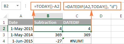
Example 4. Subtracting dates with Excel DATE function
If you prefer to supply the dates directly in the formula, then enter each date using the DATE(year, month, day) function and then subtract one date from the other.
For instance, the following formula subtracts 15-May-2015 from 20-May-2015 and returns the difference of 5 days:
=DATE(2015, 5, 20) - DATE(2015, 5, 15)

Wrapping up, when it comes to subtracting dates in Excel and you want to find out how many days are between two dates, it makes sense to go with the easiest and most obvious option - simply subtract one date directly from another.
If you are looking to count the number of months or years between two dates, then the DATEDIF function is the only possible solution and you will find a few formula examples in the next article that will cover this function in full details.
Now that you know how to subtract two dates, let's see how you can add or subtract days, months, or years to a given date. There are a number of Excel functions suitable for this purpose, and which one you use depends on which unit you want to add or subtract.
How to subtract or add days to date in Excel
If you have a date in some cell or a list of dates in a column, you can add or subtract a certain number of days to those dates using a corresponding arithmetic operation.
Example 1. Adding days to a date in Excel
The general formula to add a specified number of days to a date in as follows:
The date can be entered in several ways:
- As a cell reference, e.g.
=A2 + 10 - Using the DATE(year, month, day) function, e.g.
=DATE(2015, 5, 6) + 10 - As a result of another function. For example, to add a given number of days to the current date, use the TODAY() function:
=TODAY()+10
The following screenshot demonstrates the above formulas in action. The current date at the moment of writing was 6 May, 2015:

Note. The result of the above formulas is a serial number representing the date. To get it displayed as a date, select the cell(s) and press Ctrl+1 to open the Format Cells dialog. On the Number tab, select Date in the Category list, and then choose the date format you want. For the detailed steps, please see How to change date format in Excel.
Example 2. Subtracting days from a date in Excel
To subtract a given number of days from a certain date, you perform a usual arithmetic operation again. The only difference from the previous example is that you type the minus sign instead of plus :)
Here are a few formula examples:
=A2-10=DATE(2015, 5, 6)-10=TODAY()-10

How to add or subtract weeks to date
In case you want to add or subtract whole weeks to a certain date, you can use the same formulas as for adding / subtracting days, and simply multiply the number of weeks by 7:
Adding weeks to a date in Excel:
For example, you add 3 weeks to the date in A2, use the following formula: =A2+3*7.
Subtracting weeks from date in Excel:
To subtract 2 weeks from today's date, you write =TODAY()-2*7.
How to add / subtract months to date in Excel
If you want to add or subtract a certain number of whole months to a date, you can employ either the DATE or EDATE function, as demonstrated below.
Example 1. Add months to a date with Excel DATE function
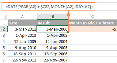
Taking a list of dates in column A for example, type the number of dates you want to add (positive number) or subtract (negative number) in some cell, say C2.
Enter the following formula in cell B2 and then drag the corner of the cell all the way down to copy the formula to other cells:
=DATE(YEAR(A2), MONTH(A2) + $C$2, DAY(A2))
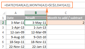
Now, let's see what the function is actually doing. The logic behind the formula is obvious and straightforward. The DATE(year, month, day) function takes the following arguments:
- the year of the date in cell A2;
- the month of the date in A2 + the number of months you specified in cell C2, and
- the day of the date in A2.
Yep, it's that simple :) If you type a negative number in C2, the formula will subtract months instead of adding them:
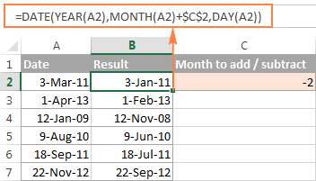
Naturally, nothing prevents you from typing the minus sign directly in the formula to subtract months from a date:
=DATE(YEAR(A2), MONTH(A2) - $C$2, DAY(A2))
And of course, you can type the number of month to add or subtract in the formula instead of referring to a cell:
=DATE(YEAR(date), MONTH(date) + N months, DAY(date))
The real formulas could look similar to these:
- Add months to date:
=DATE(YEAR(A2), MONTH(A2) + 2, DAY(A2)) - Subtract months from date:
=DATE(YEAR(A2), MONTH(A2) - 2, DAY(A2))
Example 2. Add or subtract months to a date with Excel EDATE
Microsoft Excel provides a special function that returns a date that is a specified number of months before or after the start date - the EDATE function. It is available in all versions of Excel 2007 and higher.
In your EDATE(start_date, months) formulas, you supply the following 2 arguments:
- Start_date - the start date from which to count the number of months.
- Months - the number of months to add (a positive value) or subtract (a negative value).
The following formula used on our column of dates yields exactly the same results as the DATE function in the previous example:
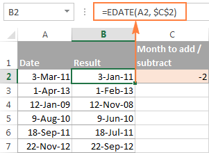
When using the EDATE function, you can also specify the start date and the number of month to add / subtract directly in the formula. Dates should be entered by using the DATE function or as results of other formulas. For example:
- To add months in Excel:
=EDATE(DATE(2015,5,7), 10)The formula adds 10 months to 7-May-2015.
- To subtract months in Excel:
=EDATE(TODAY(), -10)The formula subtracts 10 months from today's date.
Note. The Excel EDATE function returns a serial number representing the date. To force Excel to display it as a date, you should apply the Date format to the cells with your EDATE formulas. Please see Changing the date format in Excel for the detailed steps.
How to subtract or add years to date in Excel
Adding years to a date in Excel is done similarly to adding months. You use the DATE(year, month, day) function again, but this time you specify how many years you want to add:
In your Excel worksheet, the formulas may look as follows:
- To add years to a date in Excel:
=DATE(YEAR(A2) + 5, MONTH(A2), DAY(A2))The formula adds 5 years to the date in cell A2.
- To subtract years from a date in Excel:
=DATE(YEAR(A2) - 5, MONTH(A2), DAY(A2))The formula subtracts 5 years from the date in cell A2.
If you type the number of year to add (positive number) or subtract (negative number) in some cell and then refer to that cell in the DATE function, you will get a universal formula:
Add / subtract days, months and years to date
If you carefully observed the two previous examples, I think you have already guessed how to add or subtract a combination of years, months and days to a date in a single formula. Yep, using the good old DATE function :)
To add years, months, days:
To subtract years, months, days:
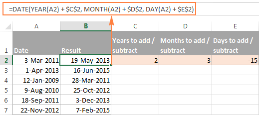
For example, the following formula adds 2 years, 3 months and subtracts 15 days from a date in cell A2:
=DATE(YEAR(A2) + 2, MONTH(A2) + 3, DAY(A2) - 15)
Applied to our column of dates, the formula takes the following shape:
=DATE(YEAR(A2) + $C$2, MONTH(A2) + $D$2, DAY(A2) + $E$2)
How to add and subtract times in Excel
In Microsoft Excel, you can add or subtract times using the TIME function. It lets you operate on time unites (hours, minutes and seconds) exactly in the same way as you handle years, months and days with the DATE function.
To add time in Excel:
To subtract time in Excel:
Where A2 contains the time value you want to change.
For example, to add 2 hours, 30 minutes and 15 seconds to the time in cell A2, you can use the following formula:
=A2 + TIME(2, 30, 15)
If you want to add and subtract time unites within one formula, just add the minus sign to the corresponding values:
=A2 + TIME(2, 30, -15)
The above formula adds 2 hours and 30 minutes to the time in cell A2 and subtracts 15 seconds.
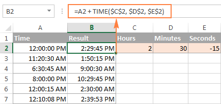
Alternatively, you can enter the time unites you want to changes in some cells, and refer to those cells in your formula:
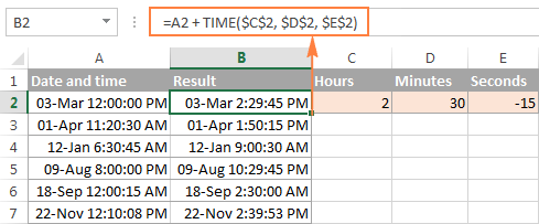
=A2 + TIME($C$2, $D$2, $E$2)
If the original cells contain both date and time, the above formula works perfectly too:
Date & Time Formula Wizard - quick way to add and subtract dates in Excel
Now that you know a bunch of different formulas to calculate dates in Excel, wouldn't you want to have just one that can do all this? Of course, such a formula can never exist. However, there exists the Date & Time Wizard that can build any formula for you on the fly, provided that you have our Ultimate Suite installed in your Excel. Here's how:
- Select the cell in which you want to insert the formula.
- Head to the Ablebits Tools tab, and click the Date & Time Wizard button:

- The Date & Time Wizard dialog window shows up. Depending on whether you want to add or subtract dates, switch to the corresponding tab, supply data for the formula arguments, and click the Insert Formula button.
As an example, let's add a few months to the date in cell A2. For this, you go to the Add tab, type A2 in the Enter a date box (or click in the box and select the cell on the sheet), and type the number of months to add in the Month box.
The wizard makes a formula and shows its preview in the cell. It also shows the calculated date under Formula result:
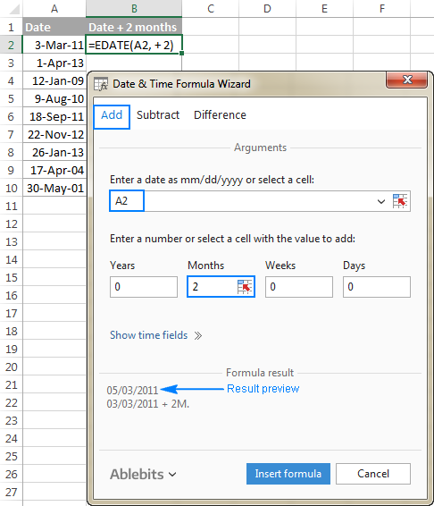
If you are satisfied with the result, click the Insert formula button. Once the formula is added, you can copy it to as many cells as necessary:

That was quite a simple formula, wasn't it? Let's give the wizard something more challenging to work on. For example, let us subtract some years, months, weeks and days from the date in A2. To have it done, switch to the Subtract tab and type the numbers in the corresponding boxes. Or you can enter the units in separate cells and supply references to those cells, as shown in the screenshot below:
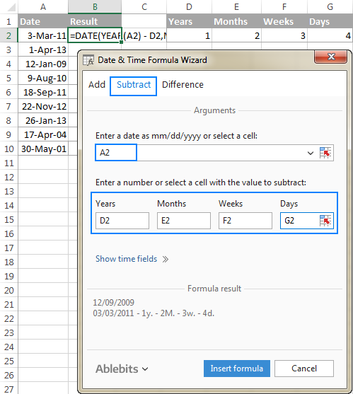
Clicking the Insert formula button inputs the following formula in A2:
=DATE(YEAR(A2)-D2,MONTH(A2)-E2,DAY(A2)-G2-F2*7)
If you plan to copy the formula to other cells, you have to change all cell references except A2 to absolute references so that the formula copies correctly (by default, the wizard always uses relative references). To fix the reference, you simply type the $ sign before the row and column coordinates, like this:
=DATE(YEAR(A2)-$D$2,MONTH(A2)-$E$2,DAY(A2)-$G$2-$F$2*7)
And get the following results:
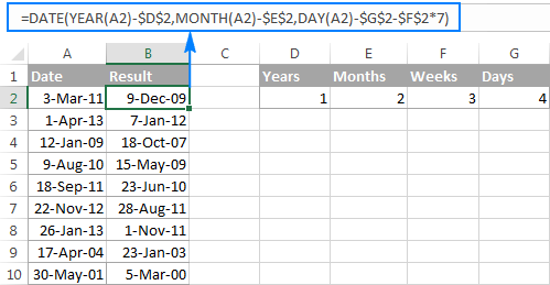
Additionally, you can click the Show time fields link and add or subtract date and time units with one formula.
If you wish to play with the Date & Time Formula Wizard in your own worksheets, you are welcome to download the 14-day trial version of the Ultimate Suite.
This is how you add and subtract dates in Excel. I am hopeful you have learned a couple of useful functions today. I thank you for reading and hope to see you on our blog next week.
 by
by
142 comments
have a set pf date in B2 need to subtract the year and want the result in year only how the do
Hi! Your explanation does not allow us to understand exactly what you want to do. However, the article above describes in detail how to subtract a year from a date. If this is not enough, please explain the problem in more detail.
I am trying to figure out how to add one number to a fiscal year so I get a list of years that look like this:
2010/11;
2011/12;
2012/13;
2013/14
And so on.
It's not that hard except I can't figure out how to do it -- every time I try it gives error messages. Any suggestions?
Hi! You can use the SEQUENCE function to create and combine two sequences of numbers. To combine numbers into a text string, use these guidelines: CONCATENATE in Excel: combine text strings, cells and columns. The formula below will do the trick for you:
=SEQUENCE(10,1,2010,1) &"/"& SEQUENCE(10,1,11,1)
Hi there! Is there a formula if I want to add several number of days in a specific column?
Column A: 03/21/24
Column B: 2 (numbers indicated in here vary from 1-4)
1= 14 days
2 = 30 days
3 = 90 days
4 = 180 days
Column C: this is where the new date will be reflected
Example:
Column A: 03/21/24
Column B: 1
Column C: 03/28/24
Thank you!
Hi! Your example does not match the description of the conditions. However, you can perform different calculations depending on the conditions if you use nested IF. Read more: Excel Nested IF statements - examples, best practices and alternatives. For example:
=IF(B1=1,A1+14,IF(B1=2,A1+30,""))
=IFS(B1=1,A1+14,B1=2,A1+30)
=CHOOSE(B1,A1+14,A1+30)
I'm using DATEIF with today and end date to get how many days due for a task. it work well if today is no later than the end date but return error when it is past the end date. I wonder if there is a way if it is past the due , the value would be 0 or negative
Hi! In the event of an error in the formula, you can use the IFERROR function to perform a new calculation. For example:
=IFERROR(DATEDIF(TODAY(),A1,"d"),DATEDIF(A1,TODAY(),"d"))
I need help with a formula to give me number of years of service. I have current day and the hire date I want the output with the number of years. I was about to add the years but that is not what i am looking for as my output answer. Can someone assist.
Hi! You can find examples and detailed instructions on how to calculate the number of years here: Excel DATEDIF function to get difference between two dates
Dear Sir
we need your support please.
how to fix this formulas,
if i will type date a cell that come to automatics Ro0.Ro1.Ro2
=IF(F8,G8<=TODAY, "NO", "RO0"))
Thank you
Hi! If I understand your task correctly, use AND or OR statement in this formula. Look for the example formulas here: Excel IF statement with multiple conditions. If this does not help, explain the problem in detail.
Hello,
I am trying to create a 60 day calculator and I want to add the option to not count specific dates. What's the best way to do this? For example, I want to calculate 60 days from May 5, 2023 but I do not want it to count days listed in columns D in the 60 days.
Thank you!
Hi! Try to use WORKDAY.INTL function. For examplle,
WORKDAY.INTL(start_date, 60, "0000000", D1:D20)
For more information, please visit: Calculating weekdays in Excel.
Hi,
I am trying to input into a particular cell the week number. and then in another Cell it would give the exact date for Saturday of the that particular week number for the year 2023.
So, for example:
in Cell A1 I put week# 2
then in Cell B2 it would give me the exact date of Saturday for the week 2 of 2023, which in this case would be 01/14/2023.
any help would be greatly appreciated!
Kind Regards,
Hi!
To use the week number to determine the day of this week, try the formula
=DATE(2023,1,1)+MIN(8-WEEKDAY(DATE(2023,1,1),2),3)+7*(D1-1)+5
Formula determines Saturday (+5 from Monday)
Hi,
I have a list of past dates or empty cells (column A). If the date in column A is within 1 year of the current date, the cell in column B should say 20. If the date is more than 1 year old, the cell in column B should say 5. And if there is no date in column A, the cell in column B should 0. Please help!
For example, using today's date:
12/16/2021 20
2/3/2021 5
12/19/2017 5
0
9/30/2022 20
0
6/22/2022 20
12/7/2018 5
0
2/19/2007 5
11/21/2021 20
8/5/2016 5
Hello!
Check an empty cell with the ISBLANK function. Use the DATEDIF function to calculate the date difference.
=IF(ISBLANK(A1),0,IF(DATEDIF(A1,TODAY(),"y")>0,5,20))
I recommend reading this guide: Calculate difference between two dates in days, weeks, months or years.
Hello,
I Have a sheet that we use as a team at my company to track the number of days of service that our clients have attended. Currently we have to do this manually because we don't provide services on Sunday. when we calculate days based on admission date - todays date it does not account for removing the Sundays. Is there a formula that can solve this?
Hello!
Use NETWORKDAYS and WORKDAY functions to calculate workdays with custom weekend parameters and holidays.
Hi, hope you can help:
A2 is a name of company
B2 is manual input of a date of delivery
In C2 I now need to add the appropriate number of days to that shown in B2 that is relevant to the name in A2 (there is a list of companies all with different number of days to be added to that entered in B2)
Hope you can advise please
Hi!
Use the VLOOKUP function to find the number of days in the list of companies that matches the required company. Use the first example in this article - Excel VLOOKUP function tutorial with formula examples. I hope I answered your question. If something is still unclear, please feel free to ask.
I am trying to create a formula where if there is a date in 1A then 1B results in a date 6 months away, but if 1A is blank then 1B stays blank.
Hi!
Use the IF function and the recommendations from this article above:
=IF(A1="","",DATE(YEAR(A1),MONTH(A1)+6,DAY(A1)))
Hi
Can you pl help me to get the Excel formula for the below
I want subtract 4 and half months (4.5) from today date
Hi!
You can only subtract days from the current date. 4.5 months is from 134 to 137 days, depending on which months it is.
Thank you.. I have not checked your previous reply
I want to Add 10 working day in every date i want to Input.. please help.. i dont much about excel
Hello!
Please check out this article to learn how to add or subtract working days to date.
Hi, I wanna ask how to create the formula for conditional format over google sheets where I want a date to change its color into red when it has reach 1 year time from that particular date written down in the cell.
for example: todays date is 27/6/22
when i insert date 31/1/22 over the cell, I want the cell to change into red color (box) when it reaches 1 year time (31/1/23).
I will be putting down more dates according the my data, so i can apply to all of them under this conditional rule, and they will change color individually according to their time in 1 year.
Thanks for your help in advance.
Hi!
The following tutorial should help: Google Sheets conditional formatting. If something is still unclear, ask a question in the comments to this article.
Greetings,
I need to create an date-alert that flags equipment for maintenance.
(Ex: Last service date was 4/15/2021. Next service date is 4/15/2022. I want a cell to change colors when the equipment is within 2 weeks of the next service date.)
Any ideas would be treasured!
JP
Hello!
The answer to your question can be found in this article: How to conditionally format dates and time in Excel - built-in rules and formulas.
I hope I answered your question.
hi,
for example:
I have a loan (6000), I wand to subtract (500) in the 27th of each month.
automatically by the system date.
thank you
Hi!
Use the DAY function to determine the day of the month.
IF(DAY(D1)=27,A1-500,A1)
I hope it’ll be helpful.
YES, Good idea but,
when:
A1=6000
B1= the formula
D1= today()
and I used this formula in B1
=IF(DAY(D1)=27,A1-500,A1)
would it continue to subtract every month? because if it false it will put A1 value after the 27th
Hi!
The formula I sent to you was created based on the description you provided in your first request. I can't guess what result you want on the 28th and beyond.
Hello,
If I have a date range, for example, 5/5/2015 - 4/30/2020 and I'd like to calculate the number of months within that range, but since the range begins on 5/5/2015 and not 5/1/2015, I would like the result to include one decimal point to represent May.
Hello!
Use the DATEDIF function to count the number of full months between dates. If I understand your task correctly, try the following formula:
=DATEDIF(A1,B1,"M")+(EOMONTH(A1,0)-A1)/30
IF i have one sheet with all users with the work date in one cell and hours in other cell and i want to present summary of the working hours spend by each user within the period by days using with formulas and not PIVOT table how to do this?? Can you help me?
Hello!
To sum values by conditions, use the SUMIFS function. Here is the article that may be helpful to you: Sum if between two dates and another criteria.
=SUMIFS(C1:C20,A1:A20,"John",B1:B20,">01-01-21",B1:B20,"<31-01-21")
This should solve your task.
Thank you a lot! Its works.
I have another issue if you can help me.
I have 2 sheets, one sheet have data for example the id, the user name, dates, hours, issues etc, and i want to the second sheet to identify with id which has issue and on which date.
can you help me with this please?
Thanks in advanced
Hello!
If you want to get a list of IDs with dates, then you need to use the FILTER function. You can find examples and instructions in this article.
I hope it’ll be helpful. If something is still unclear, please feel free to ask.
Very nice its =filter(filter(..)
Thank you ;)
Hi
I am trying to calculate the day and time difference between a start date and time and a start finish date and time for eg, start date is 12 jan 2022 15:00 and finish time is 19 January 2022 06:00.
However I can't seem to get the proper cell format to reflect day and hours in my formula cell. or get the correction function for formula to calculate and say the diff is 6 days 15 hours.
please help
Hello!
Find cell difference and use custom date and time format.
For example -
dd "d." hh "h." mm "min."
This should solve your task.