If your task is to get Excel count blank cells in your worksheet, read this article to find 3 ways to accomplish it. Learn how to search and select empty cells with the Go to Special option, use Find and Replace to count blanks or enter a formula in Excel.
In my previous post on how to count non-empty cells in Excel, I showed 3 ways to get the number of filled cells in a range. Today, you'll learn how find and count blanks in your table.
Suppose you supply goods to multiple stores. You have a worksheet in Excel with the shops' names and the quantity of items they sold. Some cells in the Items sold column are empty.
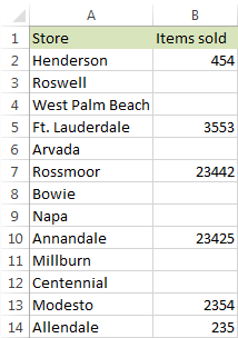
You need to make Excel count blank cells in your sheet or find and select them to see how many stores didn't provide the necessary details. Doing it manually would take too much time, so feel free to use one of the options I show in this post:
Count blank cells using Excel's Find and Replace
You can use the standard Excel Find and Replace dialog to count empty cells in your table. This tool will display the list with all blanks next to their addresses in your sheet. It also lets you navigate to any empty cell by clicking on its link in the list.
- Select the range where you need to count blank cells and press the Ctrl + F hotkey.
Note. If you select one cell Find and Replace will search the entire table.
- Leave the Find what field empty.
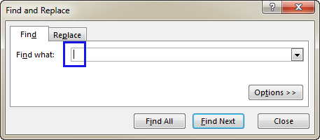
- Press Options and select the Match entire cell contents checkbox.
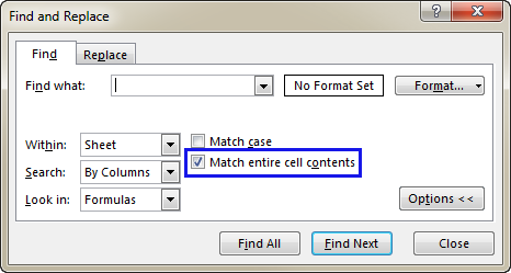
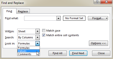
- Pick Formulas or Values from the Look in: drop-down list.
- If you choose to find Values, the tool will count all empty cells including the pseudo-blank ones.
- Select the Formulas option to search for empty cells only. You will not get cells with blank formulas or spaces.
- Press the Find All button to see the results. You will get the number of blanks in the bottom-left corner.
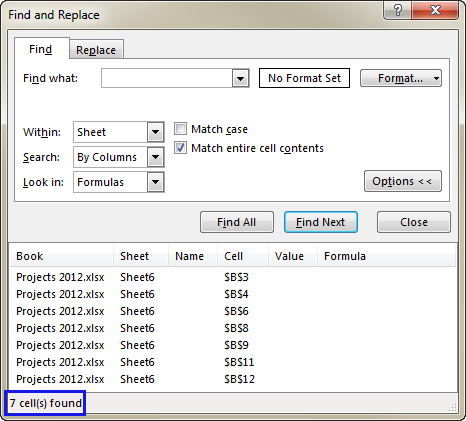
Tips:
- If you select the results on the add-in pane, it's possible to fill the empty cells with the same value, like 0 or the words "no information". To learn more, please check the article Fill empty cells with 0 or another specific value.
- If you need to quickly find all blank cells in Excel, use the Go to Special functionality as described in this article: How to find and highlight blank cells in Excel.
Excel formula for counting blank cells
This part is for the formula-oriented users. Though you will not see the found items highlighted, it's possible to get the number of blanks in any cell you select to compare to the next search.
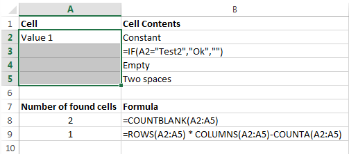
- The COUNTBLANK function will show you the number of empty cells, including the pseudo-blank ones.
- With the ROWS COLUMNS COUNTA formula, you'll get all truly empty cells. No values, no blank formulas.
Follow the steps below to apply them:
- Select any empty cell in your sheet.
- Enter one of the below formulas into the formula bar.
=COUNTBLANK(A2:A5)or
=ROWS(A2:A5) * COLUMNS(A2:A5) - COUNTA(A2:A5) - Then you can enter the range address between the brackets in your formula. Or place the mouse cursor between the brackets and manually select the necessary cell range in your sheet. You will see the address automatically appear in the formula.
- Press the Enter key.
You will get the result in the selected cell.
On the below picture, I show the summary of how these 2 formulas work with constants and pseudo-blank cells. In my sample, I have 4 cells selected. A2 has a value, A3 has a formula that returns an empty string, A4 is empty and A5 contains two spaces. Below the range, you can see the number of the found cells next to the formula I employed.
You can also use the COUNTIF formula for counting empty cells in Excel, please check out this tutorial for full details - COUNTIF for blanks and non-blanks.
Now you know how to find and count blank cells in your Excel table. Use a formula to paste the number of empty cells, turn on Find and Replace to highlight blanks, navigate to them and see their number, or choose the Go To Special feature to quickly select all blank ranges in your table. Feel free to share any other hints you may have. Be happy and excel in Excel!
 by
by
12 comments
Hello, I want to ask how to calculate blank columns and stop calculating when the next column has a filled column.
Hi! To find an empty cell in a column, use the ISBLANK function. To find the first non-empty cell, find the FALSE value using the MATCH function. For example:
=MATCH(FALSE,ISBLANK(A1:Z1),0)-1
Hope this is what you need.
Hello,
Thanks for simplifying the task. Appreciate it
I have a scenario where I need to count number of blank cells across a data range for a specific value
Column A has names of people, Columb B has a score or is blank.
I would like to excel to count the number of blank cells for each of the values in column A
Column A:
John
Mike
Cindy
Edith
Column B:
50
100
blank
80
Formula should give the result that Cindy has 1 (empty cell) to her name
Thank you.
Hi! To count the number of empty cells by condition, you can use the COUNTIFS function.
The formula might look like this:
=COUNTIFS(A1:A20,"Cindy",B1:B20,"<>"&"*")
If you want to get a list of values in column A that are matched by an empty cell in column B, you can use these instructions: Get a list of unique values based on criteria. For example:
=UNIQUE(FILTER(A1:A20,B1:B20=""))
Hi
I have client information(200 clients) with 7 columns .
I just want to delete the empty rows where all the columns are empty or without any data except the client id
How can I do this I tried Ctrl+G(but it shows all the empty cells)
I just want to delete where all the other cells are empty except the client id and name created
Thanks in advance
Hi! To correctly remove blank rows, I recommend reading these guides: How to remove all blank rows in Excel and How to delete blank rows in Excel quickly and safely.
Hi, would like to ask for help. I am trying to count blank cells where in some cells are merged. When I use Countblank formula, all merged cells are not count as 1. I wanted it to be counted as 1. Thank you!
Hi! Merging cells is only changing their format in Excel. Two merged cells are not replaced by one. Looks like this is not possible with the standard Excel options.
Hi, I would like to get formula for the following:
data are in columns A:Z, column A is to enter date in each row, columns B:Z contain random data in certain cells, mainly are empty. The formula should calculate only empty cells from last entry in each column (B:Z) referring to the last entry in column A, so how many empty cells are between last entry in column A and last entry in column B, and so on.
Thanks and regards.
Leos
Hi! You can find the row number where the last value in a column is located by using this formula:
=MAX(ROW(A1:A1000)*NOT(ISBLANK(A1:A1000)))
Hi!
I need to have o formula when I have 3 column in excel whith diferen number, for example
Colum A. Colum B. Colum C
155000 180000 3000000
For this column I have target with % for example
For Column A is 2%
For Column. B is 3%
For Column C is 4%
The limit per Column. A is 2 % for (1 - 179999)
The limit for Column B is 3% for (180000 - 299999)
The limit for Column. C is 4% for (300000 - 2000000)
How can I do this with the formul?
Hi!
I don't really understand what result you want to get. But if you have many conditions, I recommend paying attention to this article: IF AND in Excel: nested formula, multiple statements, and more. If this is not what you wanted, please describe the problem in more detail.