The tutorial explains the nuts and bolts of Excel MONTH and EOMONTH functions. You will find an array of formula examples demonstrating how to extract month from date in Excel, get the first and last day of the month, convert month name to number and more.
In the previous article, we explored a variety of formulas to calculate weekdays. Today, we are going to operate on a bigger time unit and learn the functions that Microsoft Excel provides for months.
In this tutorial, you will learn:
Excel MONTH function - syntax and uses
Microsoft Excel provides a special MONTH function to extract a month from date, which returns the month number ranging from 1 (January) to 12 (December).
The MONTH function can be used in all versions of Excel 2016 - 2000 and its syntax is as simple as it can possibly be:
Where serial_number is any valid date of the month you are trying to find.
For the correct work of Excel MONTH formulas, a date should be entered by using the DATE(year, month, day) function. For example, the formula =MONTH(DATE(2015,3,1)) returns 3 since DATE represents the 1st day of March, 2015.
Formulas like =MONTH("1-Mar-2015") also work fine, though problems may occur in more complex scenarios if dates are entered as text.
In practice, instead of specifying a date within the MONTH function, it's more convenient to refer to a cell with a date or supply a date returned by some other function. For example:
=MONTH(A1) - returns the month of a date in cell A1.
=MONTH(TODAY()) - returns the number of the current month.
At first sight, the Excel MONTH function may look plain. But look through the below examples and you will be amazed to know how many useful things it can actually do.
How to get month number from date in Excel
There are several ways to get month from date in Excel. Which one to choose depends on exactly what result you are trying to achieve.
MONTH function in Excel - get month number from date
This is the most obvious and easiest way to convert date to month in Excel. For example:
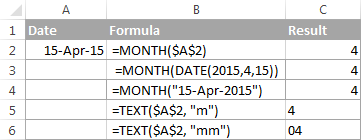
=MONTH(A2)- returns the month of a date in cell A2.=MONTH(DATE(2015,4,15))- returns 4 corresponding to April.=MONTH("15-Apr-2015")- obviously, returns number 4 too.
TEXT function in Excel - extract month as a text string
An alternative way to get a month number from an Excel date is using the TEXT function:
=TEXT(A2, "m")- returns a month number without a leading zero, as 1 - 12.=TEXT(A2,"mm")- returns a month number with a leading zero, as 01 - 12.
Please be very careful when using TEXT formulas, because they always return month numbers as text strings. So, if you plan to perform some further calculations or use the returned numbers in other formulas, you'd better stick with the Excel MONTH function.
The following screenshot demonstrates the results returned by all of the above formulas. Please notice the right alignment of numbers returned by the MONTH function (cells C2 and C3) as opposed to left-aligned text values returned by the TEXT functions (cells C4 and C5).
How to extract month name from date in Excel
In case you want to get a month name rather than a number, you use the TEXT function again, but with a different date code:
=TEXT(A2, "mmm")- returns an abbreviated month name, as Jan - Dec.=TEXT(A2,"mmmm")- returns a full month name, as January - December.

If you don't actually want to convert date to month in your Excel worksheet, you are just wish to display a month name only instead of the full date, then you don't want any formulas.
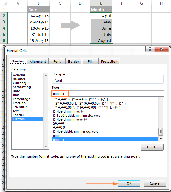
Select a cell(s) with dates, press Ctrl+1 to opent the Format Cells dialog. On the Number tab, select Custom and type either "mmm" or "mmmm" in the Type box to display abbreviated or full month names, respectively. In this case, your entries will remain fully functional Excel dates that you can use in calculations and other formulas. For more details about changing the date format, please see Creating a custom date format in Excel.
How to convert month number to month name in Excel
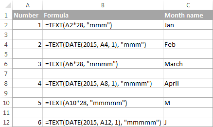
Suppose, you have a list of numbers (1 through 12) in your Excel worksheet that you want to convert to month names. To do this, you can use any of the following formulas:
To return an abbreviated month name (Jan - Dec):
=TEXT(A2*28, "mmm")
=TEXT(DATE(2015, A2, 1), "mmm")
To return a full month name (January - December):
=TEXT(A2*28, "mmmm")
=TEXT(DATE(2015, A2, 1), "mmmm")
In all of the above formulas, A2 is a cell with a month number. And the only real difference between the formulas is the month codes:
- "mmm" - 3-letter abbreviation of the month, such as Jan - Dec
- "mmmm" - month spelled out completely
- "mmmmm" - the first letter of the month name
How these formulas work
When used together with month format codes such as "mmm" and "mmmm", Excel considers the number 1 as Day 1 in January 1900. Multiplying 1, 2, 3 etc. by 28, you are getting Days 28, 56, 84, etc. of the year 1900, which are in January, February, March, etc. The format code "mmm" or "mmmm" displays only the month name.
How to convert month name to number in Excel
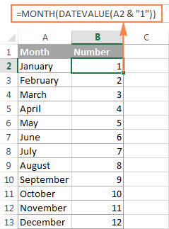
There are two Excel functions that can help you convert month names to numbers - DATEVALUE and MONTH. Excel's DATEVALUE function converts a date stored as text to a serial number that Microsoft Excel recognizes as a date. And then, the MONTH function extracts a month number from that date.
The complete formula is as follows:
=MONTH(DATEVALUE(A2 & "1"))
Where A2 in a cell containing the month name you want to turn into a number (&"1" is added for the DATEVALUE function to understand it's a date).
How to get the last day of month in Excel (EOMONTH function)
The EOMONTH function in Excel is used to return the last day of the month based on the specified start date. It has the following arguments, both of which are required:
- Start_date - the starting date or a reference to a cell with the start date.
- Months - the number of months before or after the start date. Use a positive value for future dates and negative value for past dates.
Here are a few EOMONTH formula examples:
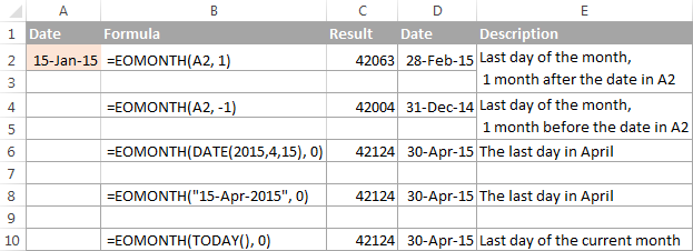
=EOMONTH(A2, 1) - returns the last day of the month, one month after the date in cell A2.
=EOMONTH(A2, -1) - returns the last day of the month, one month before the date in cell A2.
Instead of a cell reference, you can hardcode a date in your EOMONTH formula. For example, both of the below formulas return the last day in April.
=EOMONTH("15-Apr-2015", 0)
=EOMONTH(DATE(2015,4,15), 0)
To return the last day of the current month, you use the TODAY() function in the first argument of your EOMONTH formula so that today's date is taken as the start date. And, you put 0 in the months argument because you don't want to change the month either way.
=EOMONTH(TODAY(), 0)
Note. Since the Excel EOMONTH function returns the serial number representing the date, you have to apply the date format to a cell(s) with your formulas. Please see How to change date format in Excel for the detailed steps.
And here are the results returned by the Excel EOMONTH formulas discussed above:
If you want to calculate how many days are left till the end of the current month, you simply subtract the date returned by TODAY() from the date returned by EOMONTH and apply the General format to a cell:
=EOMONTH(TODAY(), 0)-TODAY()
How to find the first day of month in Excel
As you already know, Microsoft Excel provides just one function to return the last day of the month (EOMONTH). When it comes to the first day of the month, there is more than one way to get it.
Example 1. Get the 1st day of month by the month number
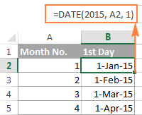
If you have the month number, then use a simple DATE formula like this:
For example, =DATE(2015, 4, 1) will return 1-Apr-15.
If your numbers are located in a certain column, say in column A, you can add a cell reference directly in the formula:
=DATE(2015, B2, 1)
Example 2. Get the 1st day of month from a date
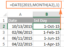
If you want to calculate the first day of the month based on a date, you can use the Excel DATE function again, but this time you will also need the MONTH function to extract the month number:
For example, the following formula will return the first day of the month based on the date in cell A2:
=DATE(2015,MONTH(A2),1)
Example 3. Find the first day of month based on the current date
When your calculations are based on today's date, use a liaison of the Excel EOMONTH and TODAY functions:
=EOMONTH(TODAY(),0) +1 - returns the 1st day of the following month.
As you remember, we already used a similar EOMONTH formula to get the last day of the current month. And now, you simply add 1 to that formula to get the first day of the next month.
In a similar manner, you can get the first day of the previous and current month:
=EOMONTH(TODAY(),-2) +1 - returns the 1st day of the previous month.
=EOMONTH(TODAY(),-1) +1 - returns the 1st day of the current month.
You could also use the Excel DATE function to handle this task, though the formulas would be a bit longer. For example, guess what the following formula does?
=DATE(YEAR(TODAY()), MONTH(TODAY()), 1)
Yep, it returns the first day of the current month.
And how do you force it to return the first day of the following or previous month? Hands down :) Just add or subtract 1 to/from the current month:
To return the first day of the following month:
=DATE(YEAR(TODAY()), MONTH(TODAY())+1, 1)
To return the first day of the previous month:
=DATE(YEAR(TODAY()), MONTH(TODAY())-1, 1)
How to calculate the number of days in a month
In Microsoft Excel, there exist a variety of functions to work with dates and times. However, it lacks a function for calculating the number of days in a given month. So, we'll need to make up for that omission with our own formulas.
Example 1. To get the number of days based on the month number
If you know the month number, the following DAY / DATE formula will return the number of days in that month:
In the above formula, the DATE function returns the first day of the following month, from which you subtract 1 to get the last day of the month you want. And then, the DAY function converts the date to a day number.
For example, the following formula returns the number of days in April (the 4th month in the year).
=DAY(DATE(2015, 4 +1, 1) -1)
Example 2. To get the number of days in a month based on date
If you don't know a month number but have any date within that month, you can use the YEAR and MONTH functions to extract the year and month number from the date. Just embed them in the DAY / DATE formula discussed in the above example, and it will tell you how many days a given month contains:
=DAY(DATE(YEAR(A2), MONTH(A2) +1, 1) -1)
Where A2 is cell with a date.
Alternatively, you can use a much simpler DAY / EOMONTH formula. As you remember, the Excel EOMONTH function returns the last day of the month, so you don't need any additional calculations:
=DAY(EOMONTH(A1, 0))
The following screenshot demonstrates the results returned by all of the formulas, and as you see they are identical:

How to sum data by month in Excel
In a large table with lots of data, you may often need to get a sum of values for a given month. And this might be a problem if the data was not entered in chronological order.
The easiest solution is to add a helper column with a simple Excel MONTH formula that will convert dates to month numbers. Say, if your dates are in column A, you use =MONTH(A2).
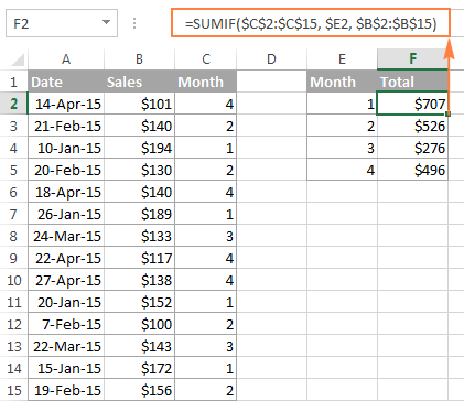
And now, write down a list of numbers (from 1 to 12, or only those month numbers that are of interest to you) in an empty column, and sum values for each month using a SUMIF formula similar to this:
=SUMIF(C2:C15, E2, B2:B15)
Where E2 is the month number.
The following screenshot shows the result of the calculations:
If you'd rather not add a helper column to your Excel sheet, no problem, you can do without it. A bit more trickier SUMPRODUCT function will work a treat:
=SUMPRODUCT((MONTH($A$2:$A$15)=$E2) * ($B$2:$B$15))
Where column A contains dates, column B contains the values to sum and E2 is the month number.
Note. Please keep in mind that both of the above solutions add up all values for a given month regardless of the year. So, if your Excel worksheet contains data for several years, all of it will be summed.
How to conditionally format dates based on month
Now that you know how to use the Excel MONTH and EOMONTH functions to perform various calculations in your worksheets, you may take a step further and improve the visual presentation. For this, we are going to use the capabilities of Excel conditional formatting for dates.
In addition to the examples provided in the above mentioned article, now I will show you how you can quickly highlight all cells or entire rows related to a certain month.
Example 1. Highlight dates within the current month
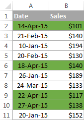
In the table from the previous example, suppose you want to highlight all rows with the current month dates.
First off, you extract the month numbers from dates in column A using the simplest =MONTH($A2) formula. And then, you compare those numbers with the current month returned by =MONTH(TODAY()). As a result, you have the following formula which returns TRUE if the months' numbers match, FALSE otherwise:
=MONTH($A2)=MONTH(TODAY())
Create an Excel conditional formatting rule based on this formula, and your result may resemble the screenshot below (the article was written in April, so all April dates are highlighted).
Example 2. Highlighting dates by month and day
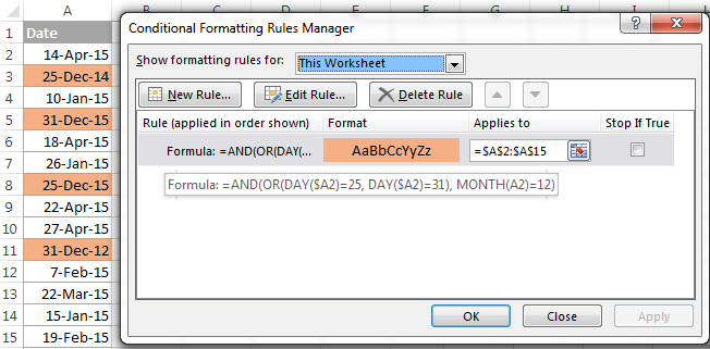
And here's another challenge. Suppose you want to highlight the major holidays in your worksheet regardless of the year. Let's say Christmas and New Year days. How would you approach this task?
Simply use the Excel DAY function to extract the day of the month (1 - 31) and the MONTH function to get the month number, and then check if the DAY is equal to either 25 or 31, and if the MONTH is equal to 12:
=AND(OR(DAY($A2)=25, DAY($A2)=31), MONTH(A2)=12)
This is how the MONTH function in Excel works. It appears to be far more versatile than it looks, huh?
In a couple of the next posts, we are going to calculate weeks and years and hopefully you will learn a few more useful tricks. If you are interested in smaller time units, please check out the previous parts of our Excel Dates series (you will find the links below). I thank you for reading and hope to see you next week!
 by
by
335 comments
I got how to take difference in two dates in months , but how to do if we need to calculate months as before15th of month consider upto previous month and vice a versa? please reply
Hello All,
I have several properties which is on rent and rent payment I'm receiving in monthly basis on different date for every property. Please advice how can I make reminder to be highlight the reminder cell date to paid, for example I must receive payment on 6th of every month My question is how I can make that every month on 6th selected cell will be highlighted example RED and after receiving of payment I can click and deselect highlighting or change to green. Thanks in advance
Hi! If I understand your task correctly, the following tutorials should help: How to conditionally format dates and time in Excel with formulas and inbuilt rules and Two ways to change background color in Excel based on cell value.
Here is an example of a formula for conditional formatting by date and by cell value:
=AND(DAY(TODAY())=6,A1=0)
Many Thanks for support will revert after implement
Please give me excel formula, of
A B C D
1 01-Jan-2016 31-Jan-2016 0M 30D C and D are wrong result
2 01-Feb-2016 26-Feb-2016 0M 25D -same-
3 27-Feb-2016 27-Feb-2016 0M 0D -same-
4 28-Feb-2016 31-Mar-2016 1M 3D -same-
Result should be in C1 1M D1 0D
C2 0M D2 26D
C3 0M D3 1D
C4 1M D4 2D
Hi! As I have written many times in the comments, the date 31-Jan-2016 means 31-Jan-2016 00:00:00. Therefore, the day 31-Jan-2016 is not included in the date difference calculation. Read more: Excel DATEDIF to calculate date difference in days, weeks, months or years.
Hi sir,how r u i want to add full month date in in one column automatically can you give me formula for that like if i put 01/02/2025 in one cell then in second cell it automatically identifies 02/02/2025 and keep following for whole month
Hi! We have a special tutorial that can help to solve your problem: How to create a sequence of dates in Excel and auto fill date series.
You can use autofill a date series, or create a sequence of dates using a formula. For example:
=SEQUENCE(EOMONTH(D1,0)-D1+1,1,D1,1)
D1 - start date.
Im trying to setup a Licence disk renuwal page.
in a1 licence paid date "2025-01-28" ,
in b1 is the actual renew month "12"
i want to have a return date in c1 2025-12-31
With this formula it gives me 2026-12-31
=EOMONTH(DATE(YEAR(A1);b1;DAY(a1));12)
Hi! If you want to get the date of the last day of the month that is less than 12 months from the paid date, try this formula:
=EOMONTH(A1,B1-1)
Hope this is what you need.
Thx
I have a spreadsheet into which I put expenditures (date, expense, for what, vendor, category, and how it was paid, cc or bank, etc). Up until now I used a separate sheet for each month, but now I would like to just use one sheet for all 12 months and then be able to pull out expenses for each category based on a particular month. I use SUMIF to total all the expenses for a category, but how would I do that based on a particular month when all the expenses for all year are in the same table? Any help you can give is appreciated.
Hello Steve!
To use the SUMIF function, you must calculate the month number in a separate column using the MONTH function. You can then use this column as a criterion in the SUMIF formula. To avoid making an additional column, try the SUMPRODUCT formula.
For example:
=SUMPRODUCT((MONTH(A2:A100)=2)*B2:B100)
i have number 6.4, 2nd is 7.9, this number is means 6year and 3 month another is 7 year and 9 month, i want to sum 6.4+7.9 = 14.1, any formla for this help me on this
Hi! If you want to write the result as a decimal number, it doesn't make sense. 14 years and 1 month will be written in the same way as 14 years and 10 months, i.e. as 14.1
Write the result in the form of text:
=IF((RIGHT(A1,1)+RIGHT(B1,1))>12, (INT(A1)+INT(B1))+INT((RIGHT(A1,1)+RIGHT(B1,1))/12)&" y "&MOD(((RIGHT(A1,1)+RIGHT(B1,1))),12)&" m", (INT(A1)+INT(B1))&" y "&((RIGHT(A1,1)+RIGHT(B1,1)))&" m")
RIGHT function will subtract the number of months from the number. MOD function will show the number of months that exceed one year. INT function will show the integer number of years.
Hi! I need to create a formula that inserts the number of the month (1-12) into a cell if the date falls between the 1st and the 15th of the month. If the date falls between the 16th and EOM, I need to put the number of the month (1-12) into another cell.
Cells in Column A are used to calculate income that is received between the 1st and 15th.
Cells in Column B are used to calculate income that is received between the 16th and EOM.
These cells will be used in a formula to determine where to add income amounts on a different sheet within the workbook.
Hi! Define the day using the DAY function. If the date is written in cell D1, the formula for column A might look like this:
=IF(DAY(D1)<16,MONTH(D1),"")
Formula for column B
=IF(DAY(D1)>15,MONTH(D1),"")
Hi,
I am trying to work out a formula if one cell = January, then another cell =31/1/24, or if the cell = February, the other cell = 28/2/24 etc for each month. Is there a simple formula for this?
Hello Thomas!
The formula below will do the trick for you:
=EOMONTH(DATE(2024,1,1), MONTH(DATEVALUE(A1&" 1"))-1)
A1 & “ 1”: combines the text “January” with the number “1” to get the text string “January 1”.
DATEVALUE(A1 & “ 1”): DATEVALUE function converts the text string “January 1” to a date.
MONTH(DATEVALUE(A1 & “ 1”)): MONTH function extracts the month number from this date.
The result is the month number for “January”, which is 1.
EOMONTH function determines the last day of the month.
Hello,
I want to find out the date of the first Friday of certain stated month, and write it in spesific cell.
For example, if first date of January stated on A1, and the date of first Friday will write in B1.
if first date of Febuary stated on A1 the the first date of Friday will appear in B1.
and so on
TQ
Hi! To get the date of the first Friday of the month, you can try this formula:
=WORKDAY.INTL(A1,1,"1111011")
You can learn more about WORKDAY.INTL function in this article: Calculating weekdays in Excel - WORKDAY and NETWORKDAYS functions.
Greetings
is it possible to use Excel to compile a list of how many Mondays, Tuesdays etc. the are for each month of a year.
Thanks
How to make automatic days of the month based on the first day of the month example 01/12/2024
Date 01, Sunday, date 02, Monday etc. until December 31
Hello Herman! If I understand your task correctly, the following formula should work for you:
="Day "&SEQUENCE(31,1,1,1)&", "&(TEXT(SEQUENCE(31,1,DATE(2024,12,1),1),"dddd"))
Use the SEQUENCE function to create a sequence of numbers. Also pay attention to these recommendations: Create a date sequence in Excel and auto fill date series. To write the date as text in the desired format, use the TEXT function.
Hello Dudley!
You can count the number of Mondays in a date range using the SUMPRODUCT formula. Create a sequence of dates from start date A1 to end date A2 using the SEQUENCE function. Determine the day of the week using the WEEKDAY function. For example:
=SUMPRODUCT(--(WEEKDAY(SEQUENCE(A2-A1+1,1,A1,1),2)=1))
Hello,
How to create a sequence of months in a certain period of time?
I have a project in a period of 3 years starting from November, so I will make November the 1st month until November 3 years later in the 36th month
Hi! Here is the guide that may be helpful to you: How to add / subtract months to date in Excel. You can create a date sequence using these instructions: Create a date sequence in Excel and auto fill date series.
The formula might look something like the following:
=EDATE(N1,SEQUENCE(36,1,0,1))
or
=EDATE(N1,ROW(A1:A36)-1)
N1 - start date.
Set the date cell to the date format that you want to use. Use these instructions: How to change Excel date format and create custom formatting.
Hello,
I have a shrinking year starting in November, so I will make November the 1st month until then the 48th month.
Hi ,
i have in excel e.g in cell A1 is Year 2024, cell A2 is January, cell B1 need to use formula to get previous year which is expected to have Year 2023, cell B2 is December.
how do i use formula to get previous year if my month is December, it does not matter which year.
if my month is in January, it should take current year.
im not sure of the formula to use.
Hi! To get the previous month's name, use the formula below:
=TEXT(EDATE(DATE(A1,MONTH(1&A2),1),-1),"mmmm")
To get the number of the month from its name, use the MONTH function. Use DATE function to create a date: the first day of this month. Use EDATE function to subtract one month from that date. Use TEXT function to get the name of the month from that date.
Use IF function to subtract 1 year from a condition. For example:
=IF(A2="January",A1-1,A1)
Or use the YEAR function:
=YEAR(EDATE(DATE(A1,MONTH(1&A2),1),-1))
Hi, thanks. How do you get the previous year using formula? for e.g. if my month is December, is there a formula to get previous year? if my month is January, then it should get current year.
so meaning by looking at the month - if it is December, then previous month, otherwise, it should get current month.
Hi! The formula I sent to you was created based on the description you provided in your first request. However, as far as I can see from your second comment, your task is now different from the original one. You can change the name of the month in the formula. I have given you all the necessary links to understand how this formula works.
Hi, I've made some changes and it works! Thanks again :)
correction:
so meaning by looking at the month - if it is December, then previous year, otherwise, it should get current year. apologies for confusion.
how do you change the date format
Hello Emmanuel!
We have a special tutorial on this. Please see: How to change Excel date format and create custom formatting.
how to convert months from the previous year to the current year.
example: April 15, 2022 to June 20, 2024 = 26 months
Hi! You can find the answer to your question in this article: Excel DATEDIF function to get difference between two dates. Try to use the formula below:
=DATEDIF(A2, B2, "m")
Sir, I have prepared the formula to calculate exact number of days between two dates (including one day fraction which do not work well in datedif formula to calculate days). Can you confirm that my formula is valid:-
SUM(IF(AND(A13=EOMONTH(A13,-1)+1,B13=EOMONTH(B13,0)),DAY(EOMONTH(A13,0))+1-DAY(A13)+DAY(B13)-DAY(EOMONTH(A13,0)))+IF(AND(A13EOMONTH(A13,-1)+1,B13=EOMONTH(B13,0)),DAY(EOMONTH(A13,0))+1-DAY(A13)+DAY(B13)-(DAY(EOMONTH(B13,0))))+(IF(AND(A13EOMONTH(A13,-1)+1,B13EOMONTH(B13,0)),IF(DAY(EOMONTH(A13,0))+1-DAY(A13)+DAY(B13)>DAY(EOMONTH(A13,0)),DAY(EOMONTH(A13,0))+1-DAY(A13)+DAY(B13)-DAY(EOMONTH(A13,0)),DAY(EOMONTH(A13,0))+1-DAY(A13)+DAY(B13))))+IF(AND(A13=EOMONTH(A13,-1)+1,B13EOMONTH(B13,0)),DAY(EOMONTH(A13,0))+1-DAY(A13)+DAY(B13)-(DAY(EOMONTH(A13,0)))))
Hi! I cannot verify this formula. It is not written completely and therefore contains errors.
I recommend reading this guide: Excel DATEDIF to calculate date difference in days, weeks, months or years.
The following formula shall for divisible month of fraction days which are left in datedif(startmonth, endmonth,"md") formula
=SUM(IF(AND((EOMONTH(A12,-1)+1)=A12,EOMONTH(B12,0)=B12),DAY(EOMONTH(B12,0)),0)+IF(AND((EOMONTH(A12,-1)+1)B12),DAY(EOMONTH(B12,0)),0)+IF(AND((EOMONTH(A12,-1)+1)<A12,EOMONTH(B12,0)B12),DAY(EOMONTH(B12,0)),0))
Suppose I want to calculate the difference of year month and date e.g. take a start date 5.6.2020 and end date 8.7.2022. The result shown by the excel is 2 years 1 month and 3 days, if we use datedif(start date, end date,"y"), datedif(start date, end date,"ym") and datedif(start date, end date,"md") formula. But, exact answer is 2 years 1 month and 4 days. Similarly, we calculate difference above fomrula between the dates 5.7.2020 and 8.8.2022, the awnser shown by the excel is 2 years 1 months and 3 days. Whereas, the correct answer should be 2 years 1 months and 5 days. I do not know how to come out of this problem. As I have to calculate salary on the basis of these dates. Please help
Hi! I have written many times that the date for example 8.7.2022 means the date and time 8.7.2022 00:00:00. You can see this by setting the cell containing the date to custom date and time format "d.mm.yyyy hh:mm:ss".
Therefore, this day cannot be included in the calculation of the number of days between two dates.
i want help with an if statement. so if the date is last day of month, to show true, other wise false. i want to do this for several dates
To get the last day of the month, use the EOMONTH function. Try this formila:
=A1=EOMONTH(A1,0)
Dear Mr.Alexander,
below sheet i want to calculate in both ways in same time. by month and by Qtr. please give me suggestion..
YR 2021 X Y X Jan mar
QTR month typ AMT AMT Q1 Q2
Q1 jan food 1.000 2.000 foodjanQ1
Q1 feb food 1.000 2.000 foodfebQ1 Food 0
Q1 mar food 1.000 2.000 foodmarQ1
Q2 apr food 2.000 3.000 foodaprQ2
Q2 may food 2.000 3.000 foodmayQ2
Q2 jun food 2.000 3.000 foodjunQ2
Q3 jul food 3.000 4.000 foodjulQ3
Q3 aug food 3.000 4.000 foodaugQ3
Q3 sep food 3.000 4.000 foodsepQ3
Q4 oct food 4.000 5.000 foodoctQ4
Q4 nov food 4.000 5.000 foodnovQ4
Q4 dec food 4.000 5.000 fooddecQ4
30.000 42.000
Thanks
Hi! If I understand your task correctly, to calculate the sum based on the condition, you can use the SUMIF or SUMIFS function. For example, to calculate the amount for Qtr.1, you can use this formula:
=SUMIF(A2:A20,"Q1",D2:D20)
You can find the examples and detailed instructions here: How to use SUMIF function in Excel with formula examples and Excel SUMIFS and SUMIF with multiple criteria.
Hi, I'm trying to find a formula to return the 15th of the next month, if the cell has a date range between 1st to 31st of the previous month. What is the best formula to use? Thank you!
Hi! To get the date on the 15th of the next month, try this formula:
=EOMONTH(A1,0)+15
Please read the above article carefully.