The tutorial shows many different ways to turn a string into a number in Excel: Convert to Number error checking option, formulas, mathematic operations, Paste Special, and more.
Sometimes values in your Excel worksheets look like numbers, but they don't add up, don't multiply and produce errors in formulas. A common reason for this is numbers formatted as text. In many cases Microsoft Excel is smart enough to convert numerical strings imported from other programs to numbers automatically. But sometimes numbers are left formatted as text causing multiple issues in your spreadsheets. This tutorial will teach you how to convert strings to "true" numbers.
How to identify numbers formatted as text in Excel
Excel has an inbuilt error checking feature that alerts you about possible problems with cell values. This appears as a small green triangle in the top left corner of a cell. Selecting a cell with an error indicator displays a caution sign with the yellow exclamation point (please see the screenshot below). Put the mouse pointer over the sign, and Excel will inform you about the potential issue: The number in this cell is formatted as text or preceded by an apostrophe.

In some cases, an error indicator does not show up for numbers formatted as text. But there are other visual indicators of text-numbers:
| Numbers | Strings (text values) |
|
|
In the image below, you can see the text representations of numbers on the right and actual numbers on the left:
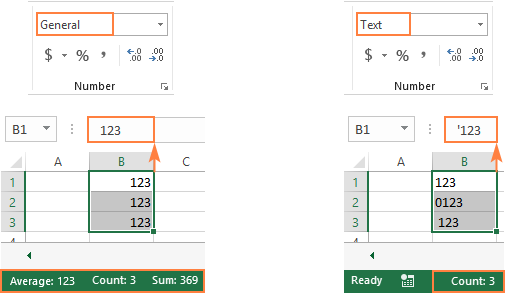
How to convert text to number in Excel
There are a handful of different ways to change text to number of Excel. Below we will cover them all beginning with the fastest and easiest ones. If the easy techniques don't work for you, please don't get disheartened. There is no challenge that cannot be overcome. You will just have to try other ways.
Convert to number in Excel with error checking
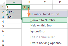
If your cells display an error indicator (green triangle in the top left corner), converting text strings to numbers is a two-click thing:
- Select all the cells containing numbers formatted as text.
- Click the warning sign and select Convert to Number.
Done!
Convert text into number by changing the cell format
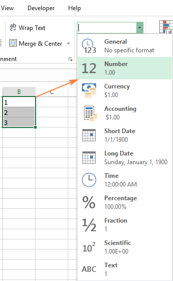
Another quick way to convert numerical values formatted as text to numbers is this:
- Select the cells with text-formatted numbers.
- On the Home tab, in the Number group, choose General or Number from the Number Format drop-down list.
Note. This method does not work in some scenarios. For example, if you apply the Text format to a cell, enter a number, and then change the cell format to Number, the cell will remain formatted as text.
Change text to number with Paste Special
Compared to the previous techniques, this method of converting text to number requires a few more steps, but works almost 100% of time.
To fix numbers formatted as text with Paste Special, here's what you do:
- Select the text-number cells and set their format to General as explained above.
- Copy a blank cell. For this, either select a cell and press Ctrl + C or right-click and choose Copy from the context menu.
- Select the cells you want to convert to numbers, right-click, and then click Paste Special. Alternatively, press the Ctrl + Alt + V shortcut.
- In the Paste Special dialog box, select Values in the Paste section and Add in the Operation section.
- Click OK.
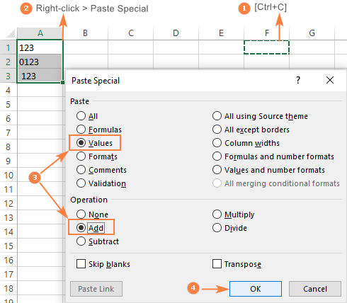
If done correctly, your values will change the default alignment from left to right, meaning Excel now perceives them as numbers.
Convert string to number with Text to Columns
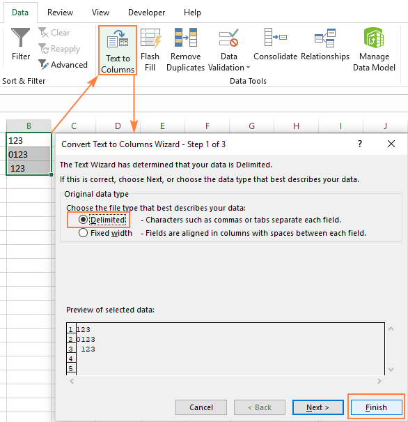
It is another formula-free way to convert text to number in Excel. When used for other purposes, for example to split cells, the Text to Columns wizard is a multi-step process. To perform the text to number conversion, you click the Finish button in the very first step :)
- Select the cells you'd like to convert to numbers, and make sure their format is set to General.
- Switch to the Data tab, Data Tools group, and click the Text to Columns button.
- In step 1 of the Convert Text to Columns Wizard, select Delimited under Original data type, and click Finish.
That's all there is to it!
Convert text to number with a formula
So far, we have discussed the built-in features that can be used to change text to number in Excel. In many situations, a conversion can be done even faster by using a formula.
Formula 1. Convert string to number in Excel
Microsoft Excel has a special function to convert a string to number - the VALUE function. The function accepts both a text string enclosed in quotation marks and a reference to a cell containing the text to be converted.
The VALUE function can even recognize a number surrounded by some "extra" characters - it's what none of the previous methods can do.
For example, a VALUE formula recognizes a number typed with a currency symbol and a thousand separator:
=VALUE("$1,000")
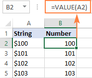
=VALUE(A2)
To convert a column of text values, you enter the formula in the first cell, and drag the fill handle to copy the formula down the column:
For more information, please see VALUE formula to convert text to number.
Formula 2. Convert string to date
Apart from text-numbers, the VALUE function can also convert dates represented by text strings.
For example:
=VALUE("1-Jan-2018")
Or
=VALUE(A2)
Where A2 contains a text-date.
By default, a VALUE formula returns a serial number representing the date in the internal Excel system. For the result to appear as an actual date, you just have to apply the Date format to the formula cell.

The same result can be achieved by using the DATEVALUE function:
=DATEVALUE(A2)
For more information, please see How to convert text to date in Excel.
Formula 3. Extract number from string
The VALUE function also comes in handy when you extract a number from a text string by using one of the Text functions such as LEFT, RIGHT and MID.
For example, to get the last 3 characters from a text string in A2 and return the result as a number, use this formula:
=VALUE(RIGHT(A2,3))
The screenshot below shows our convert text to number formula in action:
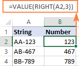
If you don't wrap the RIGHT function into VALUE, the result will be returned as text, more precisely a numeric string, which makes any calculations with the extracted values impossible.
For more information, please see How to extract number from string in Excel.
Change Excel string to number with mathematic operations
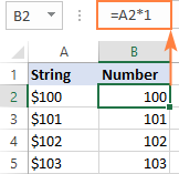
One more easy way to convert a text value to number in Excel is to perform a simple arithmetic operation that does not actually change the original value. What can that be? For example, adding a zero, multiplying or dividing by 1.
=A2+0
=A2*1
=A2/1
If the original values are formatted as text, Excel may automatically apply the Text format to the results too. You may notice that by the left-aligned numbers in the formula cells. To fix this, be sure to set the General format for the formula cells.
Tip. If you'd like to have the results as values, not formulas, use the Paste Special feature to replace formulas with their values.
That's how you convert text to number in Excel with formulas and built-in features. I thank you for reading and hope to see you on our blog next week!
 by
by
144 comments
Hi!
Referring to formula 3 (Extract number from string), I tried it on Excel, cell J4: =VALUE(RIGHT(I4,3)), with the cell I4 containing the following string of characters: "BN-675".
However, a window is displayed stating there is a problem with the formula and orienting towards typing the content with an apostrophe before the equal sign in case of not trying to type a formula.
Is there any reason the formula would not render a proper result even if it is entered correctly?
Best regards.
Hi! Could you help me to convert a text like this '100 € to number, please? I tried every method I found online but to no avail. Many thanks!
Hi! The answer to your question can be found in this guide: How to get number from any position in a string.
Hi! Note which character you are using as the function argument separator. I think in your case it is semicolon, not comma. Read more about it here: Excel formulas not working, not updating, not calculating: fixes & solutions.
Hi,
I am trying to get a SUM formula to stop showing 0. The cells it is trying to calculate form has the following formulas:
=IF(AND(K$27>=$H28,K$27<=$I28),($E28/($J28+1)),IF(K$28<$J28,0,0)).
I have tried all methods mentioned to get this to be picked up as a number, but nothing works other than hard coding.
Thanks
Sanj
Hi! The formula you wrote is not a SUM formula. It is a nested IF formula. To avoid showing 0 in the cell, you can replace the 0 in the formula with “”.
Also following tutorial should help: Display zeros as dashes or blanks
Hi Alex,
How to convert words like 'one', 'two' 'four' into numbers please?
=XMATCH(A1,{"zero","one","two","three","four","five","six","seven","eight","nine"})-1
Hello Diana!
You can convert words to numbers either by using a nested IF statement or by using a VBA macro. For example:
=IF(A1="one",1,IF(A1="two",2,""))
Thank you :)
I want to add number of time an alphanumeric appears in a row or column but excel is counting the column instead of number it appears.
For example: in column A1:A100, we have the followings: 3P+2P+1P+1P+1P+3P+2P+3P+1P
using:
=countif(A1:A100,">=1P")
the result is:
=9
But the result i was hoping to get should be: 17
Can you help with the formulae please.
Hello Joseph!
Your formula counts the number of values, not the sum of the values. Learn more about how the COUNTIF function works: COUNTIF function in Excel - count if not blank, greater than, duplicate or unique.
You cannot sum these numbers because they are written in a text string. Extract these numbers into a new column as described in the instructions: How to extract number from string in Excel.
Then you will be able to do the summation.
Not sure if there is a solution here but here goes.
I'm trying (ultimately) create a list box of particular values (numeric).
Say there is a value I refer to as "Sheet Yield". It is a number in a cell. Say it is 80.
I then want to create a list box that can populate itself with "1-80" or "1 through 'Sheet Yield'"
I need to reference either within a formula the hard coded 80 as an input/reference and return a numeric list of each value between the 2.
I don't want to reference any cells in the worksheet, or have to manually key then in the spreadsheet to use or reference them.
So it's like taking say, the value in a Named Range or just a beginning and ending number, hopefully by just referencing a variable or name.
If that can be done I want to attach the numbers to a list box. To this list box I would then iterate/append to the previous set an additional set of numbers, thereby expanding the selections in the list box.
Probably sounds a bit strange but curious how I'd go about doing this. Wracking my brain. Thanks if you have ideas!
John
Hello John!
If I understand the problem correctly, you can name the cell that creates the dropdown list of desired values. Then use that name in the SEQUENCE formula. For example:
=SEQUENCE(end-start,1,start,1)
Maybe this article will help: Excel named range - how to define and use names in Excel.
How to remove extra space from excel?
Hi! If I understand your task correctly, the following tutorial should help: 3 ways to remove spaces between words / numbers in Excel cells.
How to convert 12,34.00 to 1,234.00 or to 1234?
Hi! You can find the examples and detailed instructions here: How to extract number from string in Excel. The formula might look like this:
=SUMPRODUCT(MID(0&A1, LARGE(INDEX(ISNUMBER(--MID(A1, ROW(INDIRECT("1:"&LEN(A1))), 1)) * ROW(INDIRECT("1:"&LEN(A1))), 0), ROW(INDIRECT("1:"&LEN(A1))))+1, 1) * 10^ROW(INDIRECT("1:"&LEN(A1)))/10)
or
=TEXTJOIN("",TRUE,IFERROR(--MID(A1,ROW(INDIRECT("1:"&LEN(A1))),1),""))
You can delete the last two characters using LEFT function. For example:
=LEFT(TEXTJOIN("",TRUE,IFERROR(--MID(A1,ROW(INDIRECT("1:"&LEN(A1))),1),"")), LEN(TEXTJOIN("",TRUE,IFERROR(--MID(A1,ROW(INDIRECT("1:"&LEN(A1))),1),"")))-2)
Hi,
I need to copy 5 digit numbers with leading zeros and paste them into our account software. I can see they have zeros in front of them but when I copy and paste even in excel they lose their zeros again. I changed them to numbers with different methods but none is working. Please can you help, many thanks.
Hello Tina!
To copy the text “00777” to Excel without it being automatically converted to the number “777,” you can use one of the following methods:
Method 1: Use an Apostrophe
Copy the text “00777”.
In Excel: Click on the cell where you want to paste the text.
Paste with Apostrophe: Type an apostrophe (') before pasting the text. For example, type '00777. The apostrophe tells Excel to treat the entry as text.
Method 2: Format Cells as Text
In Excel: Select the cells where you want to paste the text.
Format as Text: Right-click on the selected cells and choose “Format Cells”. In the dialog box, select “Text” and click “OK”.
Paste the Text: Now paste the text “00777” into the formatted cells. Excel will treat it as text and preserve the leading zeros.
Method 3: Use Paste Special
Copy the text “00777”.
In Excel: Right-click on the cell where you want to paste the text.
Paste Special: Choose “Paste Special” and then select “Text”. Click “OK” to paste the text as is.
These methods will ensure that the text “00777” is not converted to the number “777” in Excel.
On a daily basis I am downloading hourly weather data from a government website (NOAA), and I am looking to obtain the extremes (highs/lows) from the downloaded data. Since this information comes downloaded as text, I have to convert that text to values (which is easy enough). However, not all the hours over the 24-hour period have values. For example, in the mornings and evenings, there may not be a Heat Index ... therefore this data appears as a blank cell when downloaded into Excel. When I convert the hourly data of these blank cells to a value, they come back as "#VALUE!" indicating an error. I cannot figure out how to find the error or get these blank cells to actually return as blank ... which throws my follow-on calculations off.
Hi! If you convert a blank cell to a number, you won't get any error. My guess is that these cells have either a space or some non-printable characters. I don't know what method you use for converting these cells into numbers. If you are using a formula, have a look at the IFERROR function. For example:
=IFERROR(VALUE(A1),"")
You can also find useful information in this article: How to remove special (unwanted) characters from string in Excel
You can solve the problem without using formulas. Pay attention to the Convert Text tool. Convert numbers stored as text to the correct number format. Replace unwanted characters and line breaks with the ones you need, and convert accented characters to their non-accented equivalents. It is available as a part of our Ultimate Suite for Excel that you can install in a trial mode and check how it works for free.
Thanks!
The information pulled in from NOAA is through Excel's Data/Query tools from tables on the NOAA website.
It all worked! Thanks!
Hi there, I'm trying to create a spreadsheet that auto calculates my monthly business mileage depending on which location I work at each day (4 different locations) using "IF" with multiple text data representing the return mileage to each location (hope that makes sense):
=IF(B3="GRV", "36.8", IF(B3="CTM", "9.4", IF(B3="RTR", "11.8", IF(B3="GLM", "10.4", "RD"))))
If I am not working at any of the locations, this is recorded as Rest Day (RD).
I have created the formula to calculate the mileage in each row, but now need to add up the total mileage. However, as the mileage in each row is showing as Text, Autosum doesn't work, so I need another way to do this. When reading all your solutions above, none of these seem to apply as I already have the IF formula, and can't see a way to extract just the numbers from the mileage column.
Would appreciate any advice you can offer, thanks, Carlos, UK.
Scratch that, I've managed to resolve it from another post in your comments!!
I removed the quotes around the numbers, formatted the cells to Numbers, and hey presto!!
=IF(B2="GRV", 36.8, IF(B2="CTM", 9.4, IF(B2="RTR", 11.8, IF(B2="GLM", 10.4, "RD"))))
Thank you for your solution, even if it wasn't directly for me lol. Really do appreciate people like you who put so much effort into helping others.
Regards, Carlos.
Hello. Suppose I have categories in the column
ex: Sex: M or F. How do I encode that so that it shows as 1 or 2. or any other number? thank you
Hi! You can't replace a letter with a number using formatting. You can set the value to 1 or 2 in another cell using the IF function.
I am having an issue when attempting to do a sum total of a column of numbers.
The figures in the column are the result of a formula =IF(C3="Full", "£88", IF(C3="Half", "£44",))
The corresponding £88 & £44 do not then appear in the =SUM(D3:D33)
Can you recommend a work around?
Hi! Your formulas return text, not a number. Therefore, the SUM function does not work. You can return numbers from an IF formula and apply a financial format to the cell to show the currency symbol.
=IF(C3="Full", 88, IF(C3="Half", 44,))
Read more about number formats here: Custom Excel number format.
This resolved my issue, Thank you!!
i used the MS365 app to scan and then "image to TABLE" function to pull in some text and numbers from a hardcopy sheet. this has worked however the numbers in the cells seem to be in accountancy format (maybe a red herring) but none of the above solutions will convert them into real number so I can manipulate them. Only way is to overwrite the number in the cells, however I have hundreds of numbers to convert, is there another solution that i can try?
Thanks
Hi! To convert your text to a number, try to use Convert text tool. It is available as a part of our Ultimate Suite for Excel that you can install in a trial mode and check how it works for free.
Thank you so much! None of the other ways worked, only the "convert" from Ablebits Data
how to convert 05.30 to 0530?
Hi! Here is the article that may be helpful to you: How to remove characters/text from string in Excel.
The formula might look like this:
=SUBSTITUTE(A1,".","")
I have a number like ex.
4512
652
1843
4756
8543
1549
7643
94785
and the total of 1st, 3rd and 8th Number is 101140
But the is converted in Value (No use of Trace Precedents Option) There is no same Total and come by any other number.
Show the formula which help me to to know that 1st 3rd and 8th Option are included in 101140 Total
Hi! Maybe this article will be helpful: How to find all combinations of numbers that equal given sum in Excel.
I have already tried something like 10 methods to convert cells like this
1 959,94
(where the space is the thousand separator and the comma is the decimal separator) to numbers, but nothing has worked. What would work?
It works
=VALUE(CONCAT(TEXTSPLIT(CONCAT(TEXTSPLIT(A1," ")), ",")))/100
Try this
=VALUE(CONCAT(TEXTSPLIT(CONCAT(TEXTSPLIT(A1," ")), ",")))
I got it just by typing
=[cell with number in text format]+0
After exhausting all the methods I could find on the web, I solved the problem by copying and pasting the problematic data to MS Word, then re-exporting to Excel as Text. It was immediately recognizable by Excel as values for purposes of applying formulas, summation, etc.
this works for me. thanks for your input
this is not working in any of the solutions/function provided above . the excel i have uses "," for thousand separator and "." for decimals
2.866.794,97
321.279,70
321.279,70
45.647,28
45.647,28
Hi!
For the above methods to work, the number separators must match the default decimal separator and thousand separator that is specified in the Windows Reginal Settings.
Please have a look at this article – How to change Excel CSV delimiter to comma or semicolon.
I want to convert from this value 1-120-00001297-7 to 1120000012977. How can i do? Thank you.
Hello!
You can find the examples and detailed instructions here: How to remove characters/text from string in Excel.
I hope it’ll be helpful.
Great explanation, thank you
I encounter this problem with different way, I downlaoded a sheet that includes column "Budget", the cells in this colum are formatted as currency and it is left aligned, and the status bar shows only count. I tried to convert it to numbe by using Value function but it gives me error, the only way that worked with me, is selecting the cells and replace $ to blank, this makes the figures inside the cells numbers.
Is there any explanation for this?
Hello!
The $ sign in the cell was not obtained using number formatting. It is written as text. So when you remove it, the value becomes a number.