In this quick lesson, you will learn how to filter in Excel dynamically with formulas. Examples to filter duplicates, cells containing certain text, with multiple criteria, and more.
How do you usually filter in Excel? For the most part, by using Auto Filter, and in more complex scenarios with Advanced Filter. Being fast and powerful, these methods have one significant drawback - they do not update automatically when your data changes, meaning you would have to clean up and filter again. The introduction of the FILTER function in Excel 365 becomes a long-awaited alternative to the conventional features. Unlike them, Excel formulas recalculate automatically with each worksheet change, so you'll need to set up your filter just once!
Excel FILTER function
The FILTER function in Excel is used to filter a range of data based on the criteria that you specify.
The function belongs to the category of Dynamic Arrays functions. The result is an array of values that automatically spills into a range of cells, starting from the cell where you enter a formula.
The syntax of the FILTER function is as follows:
Where:
- Array (required) - the range or array of values that you want to filter.
- Include (required) - the criteria supplied as a Boolean array (TRUE and FALSE values).
Its height (when data is in columns) or width (when data is in rows) must be equal to the that of the array argument. - If_empty (optional) - the value to return when no entries meet the criteria.
The FILTER function is only available in Excel for Microsoft 365 and Excel 2021. In Excel 2019, Excel 2016 and earlier versions, it is not supported.
Basic Excel FILTER formula
For starters, let's discuss a couple of very simple cases just to gain more understanding how an Excel formula to filter data works.
From the below data set, supposing you want to extract the records with a specific value in the Group, column, say group C. To have it done, we supply the expression B2:B13="C" to the include argument, which will produce a required Boolean array, with TRUE corresponding to "C" values.
=FILTER(A2:C13, B2:B13="C", "No results")
In practice, it's more convenient to input the criteria in a separate cell, e.g. F1, and use a cell reference instead of hardcoding the value directly in the formula:
=FILTER(A2:C13, B2:B13=F1, "No results")
Unlike Excel's Filter feature, the function does not make any changes to the original data. It extracts the filtered records into the so-called spill range (E4:G7 in the screenshot below), beginning in the cell where the formula is entered:
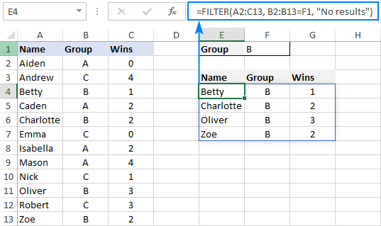
If no records match the specified criteria, the formula returns the value you put in the if_empty argument, "No results" in this example:
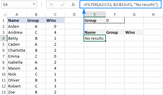
If you'd rather return nothing in this case, then supply an empty string ("") for the last argument:
=FILTER(A2:C13, B2:B13=F1, "")
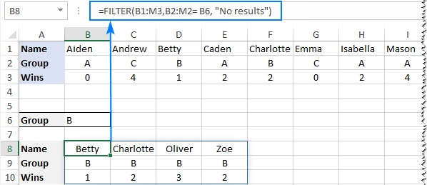
In case your data is organized horizontally from left to right like shown in the screenshot below, the FILTER function will work nicely too. Just make sure you define appropriate ranges for the array and include arguments, so that the source array and Boolean array have the same width:
=FILTER(B2:M4, B3:M3= B7, "No results")
Excel FILTER function - usage notes
To effectively filter in Excel with formulas, here are a couple of important points to take notice of:
- The FILTER function automatically spills the results vertically or horizontally in the worksheet, depending on how your original data is organized. So, please make sure you always have enough empty cells down and to the right, otherwise you'll get a #SPILL error.
- The results of the Excel FILTER function are dynamic, meaning they update automatically when values in the original data set change. However, the range supplied for the array argument is not updated when new entries are added to the source data. If you wish the array to resize automatically, then convert it to an Excel table and build formulas with structured references, or create a dynamic named range.
How to filter in Excel - formula examples
Now that you know how a basic Excel filter formula works, it's time to get some insights into how it could be extended for solving more complex tasks.
Filter with multiple criteria (AND logic)
To filter data with multiple criteria, you supply two or more logical expressions for the include argument:
The multiplication operation processes the arrays with the AND logic, ensuring that only the records that meet all the criteria are returned. Technically, it works this way:
The result of each logical expression is an array of Boolean values, where TRUE equates to 1 and FALSE to 0. Then, the elements of all the arrays in the same positions are multiplied. Since multiplying by zero always gives zero, only the items for which all the criteria are TRUE get into the resulting array, and consequently only those items are extracted.
The below examples show this generic formula in action.
Example 1. Filter multiple columns in Excel
Extending our basic Excel FILTER formula a little further, let's filter the data by two columns: Group (column B) and Wins (column C).
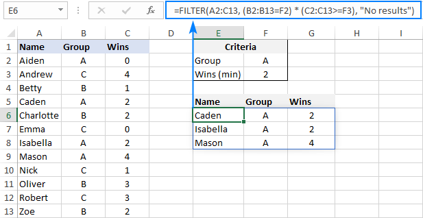
For this, we set up the following criteria: type the name of the target group in F2 (criteria1) and the minimum required number of wins in F3 (criteria2).
Given that our source data is in A2:C13 (array), groups are in B2:B13 (range1) and wins are in C2:C13 (range2), the formula takes this form:
=FILTER(A2:C13, (B2:B13=F2) * (C2:C13>=F3), "No results")
As the result, you get a list of players in group A who have secured 2 or more wins:
Example 2. Filter data between dates
First off, it should be noted that it's not possible to make up a generic formula to filter by date in Excel. In different situations, you will need to build criteria differently, depending on whether you want to filter by a specific date, by month, or by year. The purpose of this example is to demonstrate the general approach.
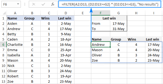
To our sample data, we add one more column containing the dates of the last win (column D). And now, we will extract the wins that occurred in a specific period, say between May 17 and May 31.
Please notice that in this case, both criteria apply to the same range:
=FILTER(A2:D13, (D2:D13>=G2) * (D2:D13<=G3), "No results")
Where G2 and G3 are the dates to filter between.
Filter with multiple criteria (OR logic)
To extract data based on multiple OR condition, you also use logical expressions like shown in the previous examples, but instead of multiplying, you add them up. When the Boolean arrays returned by the expressions are summed, the resulting array will have 0 for entries that do not meet any criteria (i.e. all the criteria are FALSE), and such entries will be filtered out. The entries for which at least one criterion is TRUE will be extracted.
Here's the generic formula to filter columns with the OR logic:
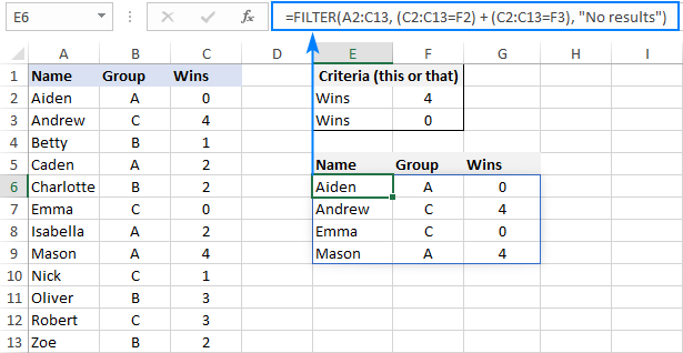
As an example, let's extract a list of players that have this or that number of wins.
Assuming the source data is in A2:C13, wins are in C2:C13, and the win numbers of interest are in F2 and F3, the formula would go as follows:
=FILTER(A2:C13, (C2:C13=F2) + (C2:C13=F3), "No results")
As the result, you know which players have won all the games (4) and which have won none (0):
Filter based on multiple AND as well as OR criteria
In situation when you need to apply both criteria types, remember this simple rule: join the AND criteria with asterisk (*) and OR criteria with the plus sign (+).
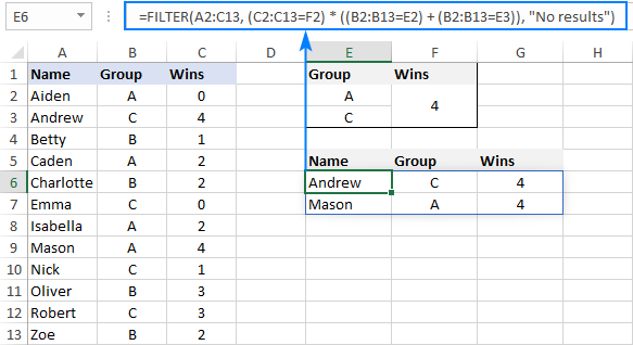
For example, to return a list of players that have a given number of wins (F2) AND belong to the group mentioned in either E2 OR E3, build the following chain of logical expressions:
=FILTER(A2:C13, (C2:C13=F2) * ((B2:B13=E2) + (B2:B13=E3)), "No results")
And you will get the following result:
How to filter duplicates in Excel
When working with huge worksheets or combining data from different sources, there's often a possibility that some duplicates would sneak in.
If you are looking to filter out duplicates and extract unique items, then use the UNIQUE function as explained in the above linked tutorial.
If your goal is to filter duplicates, i.e. extract entries that occur more than once, then use the FILTER function together with COUNTIFS.
The idea is to get the occurrences counts for all the records and extract those greater than 1. To get the counts, you supply the same range for each criteria_range / criteria pair of COUNTIFS like this:
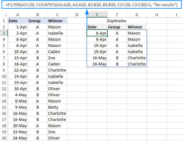
For example, to filter duplicate rows from the data in A2:C20 based on the values in all 3 columns, here's the formula to use:
=FILTER(A2:C20, COUNTIFS(A2:A20, A2:A20, B2:B20, B2:B20, C2:C20, C2:C20)>1, "No results")
Tip. To filter duplicates based on the values in the key columns, include only those specific columns in the COUNTIFS function.
How to filter out blanks in Excel
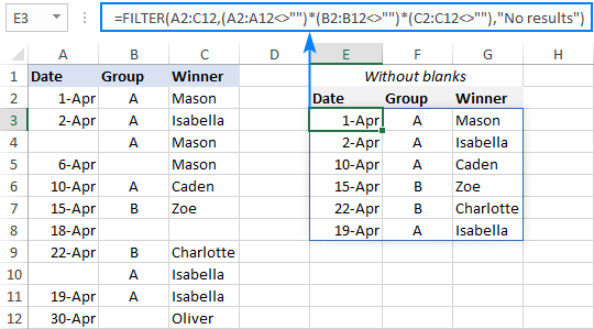
A formula for filtering out blank cells is, in fact, a variation of the Excel FILTER formula with multiple AND criteria. In this case, we check whether all (or particular) columns have any data in them and exclude the rows where at least one cell is empty. To identify non-blank cells, you use the "not equal to" operator (<>) together with an empty string ("") like this:
With the source data in A2:C12, to filter out rows containing one or more blank cells, the following formula is entered in E3:
Filter cells containing specific text
To extract cells that contain certain text, you can use the FILTER function together with the classic If cell contains formula:
Here's how it works:
- The SEARCH function looks for a specified text string in a given range and returns either a number (the position of the first character) or #VALUE! error (text not found).
- The ISNUMBER function converts all the numbers to TRUE and errors to FALSE and passes the resulting Boolean array to the include argument of the FILTER function.
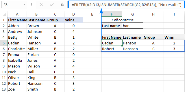
For this example, we've added the Last names of players in B2:B13, typed the part of the name we want to find in G2, and then use the following formula to filter the data:
=FILTER(A2:D13, ISNUMBER(SEARCH(G2, B2:B13)), "No results")
As the result, the formula retrieves the two surnames containing "han":
Filter and calculate (Sum, Average, Min, Max, etc.)
A cool thing about the Excel FILTER function is that it can not only extract values with conditions, but also summarize the filtered data. For this, combine FILTER with aggregation functions such as SUM, AVERAGE, COUNT, MAX or MIN.
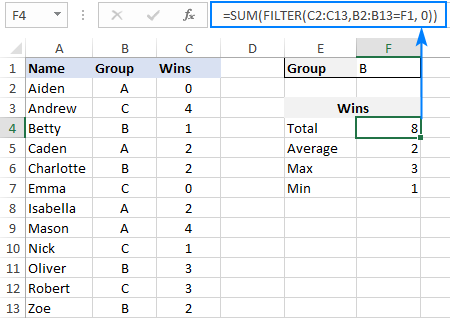
For instance, to aggregate data for a specific group in F1, use the following formulas:
Total wins:
=SUM(FILTER(C2:C13, B2:B13=F1, 0))
Average wins:
=AVERAGE(FILTER(C2:C13, B2:B13=F1, 0))
Maximum wins:
=MAX(FILTER(C2:C13, B2:B13=F1, 0))
Minimum wins:
=MIN(FILTER(C2:C13, B2:B13=F1, 0))
Please pay attention that, in all the formulas, we use zero for the if_empty argument, so the formulas would return 0 if no values meeting the criteria are found. Supplying any text such as “No results” would result in a #VALUE error, which is obviously the last thing you want :)
Case-sensitive FILTER formula
A standard Excel FILTER formula is case-insensitive, meaning it makes no distinction between lowercase and uppercase characters. To distinguish text case, nest the EXACT function in the include argument. This will force FILTER to do logical test in a case-sensitive manner:
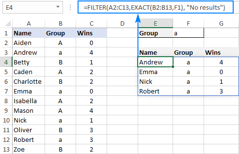
Supposing, you have both groups A and a and wish to extract records where the group is the lowercase "a". To have it done, use the following formula, where A2:C13 is the source data and B2:B13 are groups to filter:
=FILTER(A2:C13, EXACT(B2:B13, "a"), "No results")
As usual, you can input the target group in a predefined cell, say F1, and use that cell reference instead of hardcoded text:
=FILTER(A2:C13, EXACT(B2:B13, F1), "No results")
How to FILTER data and return only specific columns
For the most part, filtering all columns with a single formula is what Excel users want. But if your source table contains tens or even hundreds of columns, you may certainly want to limit the results to a few most important ones.
Example 1. Filter some adjacent columns
In situation when you want some neighboring columns to appear in a FILTER result, include only those columns in array because it is this argument that determines which columns to return.
In the basic FILTER formula example, supposing you wish to return the first 2 columns (Name and Group). So, you supply A2:B13 for the array argument:
=FILTER(A2:B13, B2:B13=F1, "No results")
As the result, we get a list of participants of the target group defined in F1:

Example 2. Filter non-adjacent columns
To cause the FILTER function to return non-contiguous columns, use this clever trick:
- Make a FILTER formula with the desired condition(s) using the entire table for array.
- Nest the above formula inside another FILTER function. To configure the "wrapper" function, use an array constant of TRUE and FALSE values or 1's and 0's for the include argument, where TRUE (1) marks the columns to be kept and FALSE (0) marks the columns to be excluded.
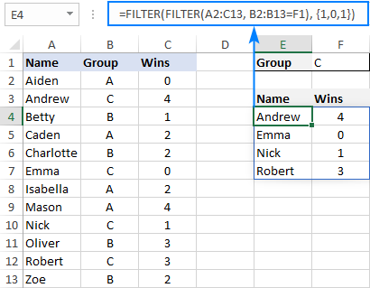
For example, to return only Names (1st column) and Wins (3rd column), we are using {1,0,1} or {TRUE,FALSE,TRUE} for the include argument of the outer FILTER function:
=FILTER(FILTER(A2:C13, B2:B13=F1), {1,0,1})
Or
=FILTER(FILTER(A2:C13, B2:B13=F1), {TRUE,FALSE,TRUE})
How to limit the number of rows returned by FILTER function
If your FILTER formula finds quite a lot of results, but your worksheet has limited space and you cannot delete the data below, then you can limit the number of rows the FILTER function returns.
Let's see how it works on an example of a simple formula that pulls players from the target group in F1:
=FILTER(A2:C13, B2:B13=F1)
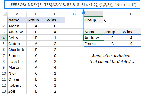
The above formula outputs all the records that it finds, 4 rows in our case. But suppose you just have space for two. To output only the first 2 found rows, this is what you need to do:
- Plug the FILTER formula into the array argument of the INDEX function.
- For the row_num argument of INDEX, use a vertical array constant like {1;2}. It determines how many rows to return (2 in our case).
- For the column_num argument, use a horizontal array constant like {1,2,3}. It specifies which columns to return (the first 3 columns in this example).
- To take care of possible errors when no data matching your criteria is found, you can wrap your formula in the IFERROR function.
The complete formula takes this form:
=IFERROR(INDEX(FILTER(A2:C13, B2:B13=F1), {1;2}, {1,2,3}), "No result")
When working with large tables, writing array constants manually may be quite cumbersome. No problem, the SEQUENCE function can generate the sequential numbers for you automatically:
=IFERROR(INDEX(FILTER(A2:C13, B2:B13=F1), SEQUENCE(2), SEQUENCE(1, COLUMNS(A2:C13))), "No result")
The first SEQUENCE generates a vertical array containing as many sequential numbers as specified in the first (and only) argument. The second SEQUENCE uses the COLUMNS function to count the number of columns in the dataset and produces an equivalent horizontal array.
Tip. To return data from specific columns, not all the columns, in the horizontal array constant that you use for the column_num argument of INDEX, include only those specific numbers. For instance, to extract data from the 1st and 3rd columns, use {1,3}.
Excel FILTER function not working
In situation when your Excel FILTER formula results in an error, most likely that will be one of the following:
#CALC! error
Occurs if the optional if_empty argument is omitted, and no results meeting the criteria are found. The reason is that currently Excel does not support empty arrays. To prevent such errors, be sure to always define the if_empty value in your formulas.
#VALUE error
Occurs when the array and include argument have incompatible dimensions.
#N/A, #VALUE, etc.
Different errors may occur if some value in the include argument is an error or cannot be converted to a Boolean value.
#NAME error
Occurs when trying to use FILTER in an older version of Excel. Please remember that it is a new function, which is only available in Office 365 and Excel 2021.
In new Excel, a #NAME error occurs if you accidentally misspell the function's name.
#SPILL error
Most often, this error occurs if one or more cells in the spill range are not completely blank. To fix it, just clear or delete non-empty cells. To investigate and resolve other cases, please see #SPILL! error in Excel: what it means and how to fix.
#REF! error
Occurs when a FILTER formula is used between different workbooks, and the source workbook is closed.
That's how to filer data in Excel dynamically. I thank you for reading and hope to see you on our blog next week!
Download practice workbook
Filter in Excel with formulas (.xlsx file)
 by
by
336 comments
Hi all,
Can I get excel to give me just the sum of all customer invoices amounts when using a filter function?
In my example below, I have invoices amounts in column C, customer name in column A and Division in Column B. I use the formula:
=FILTER($C$5:$E$24;$D$5:$D$24="Apples") to get only the division "Apples". And it gives me every single invoice amount filtered only by Apples Division:
Customer A Apples 345,45
Customer A Apples 25547,84
Customer A Apples 72484,25
Customer A Apples 110138,91
Customer A Apples 44126,78
Customer A Apples 41589,27
Customer B Apples 5598,9
Customer B Apples 3345,12
Customer B Apples 3467,4
Customer E Apples 67144,25
Customer E Apples 94669,85
But I need the formula to give me only the sum by customer, like this:
Customer A Apples 294232,5
Customer B Apples 12411,42
Customer E Apples 161814,1
How can I enhance the formula to have that? Thank you all for the support.
Original table:
Customer Name Division Amoun in EUR
Customer A Apples 345,45
Customer A Apples 25547,84
Customer A Apples 72484,25
Customer A Apples 110138,91
Customer A Apples 44126,78
Customer A Apples 41589,27
Customer B Apples 5598,9
Customer B Apples 3345,12
Customer B Apples 3467,4
Customer C Oranges 21417,38
Customer D Oranges 18067,22
Customer D Oranges 4841,43
Customer E Apples 67144,25
Customer E Apples 94669,85
Customer F Oranges 21559,38
Customer F Oranges 23064,48
Customer F Oranges 22759,69
Customer G Oranges 17558,31
Customer G Oranges 12219,43
Customer G Oranges 39779,94
Hello! To calculate an amount for two or more conditions, try the SUMIFS function. Here are the detailed instructions: How to use Excel SUMIFS and SUMIF with multiple criteria.
For example:
=SUMIFS(C1:C20,A1:A20,"Customer A",B1:B20,"Apples")
I have a workbook where I use the FILTER function in order to make a filter from 16.000 entries from a worksheet to another one, by some criteria and It work just fine on my version (365).
My problem is that the other guys from my department have Excel older versions (previous than 2021).
When they open the file in their computers, immediately gives a error (#name) on the destiny filter worksheet.
I'm trying to manage some VBA Code in order to block calculation on the destiny worksheet (where the FILTER function is set) if the file is open is Excel versions previous than 2021, but so far I was not able to do it.
I appreciate any help that you can give to me.
Hi!
Try using a pivot table instead of the FILTER function. You will also be able to get some of the data by some criterion. Read more: How to make and use Pivot Table in Excel.
Hi
Thanks for your reply.
I canno't implement your solution because the destiny worksheet is shared with other department and they canno't have access to all the entries.
It could be protected, preventing them do change the criterion, but then would not refresh the pivot table.
Still working on the solution :)
Hello,
Why my filter formula stop working ?
I use this formula:
=FILTER(FILTER(Log!A2:P200,(Log!A2:A200"completed")*(Log!C2:C200="yes"),"Nothing Found"),{0,0,0,1,1,1,1,0,0,1,0,0,0,0,0,1})
one is working fine, I get everything I am filtering from my Log tab, next day is no working anymore.
It is either only filtering the first 4 rows or none at all.
I have to redo the formula again, over and over.
Anyone know why this happens and how to fix it?
Hi!
I can't check the formula that contains unique references to your workbook worksheets. I don't have your data.
(Log!A2:A200"completed") as your first logical argument should probably be 200="
Thanks for this review of the Filter Formula options.
I am having an issue with a worksheet that has a filter and I also want dynamic print area. looking for suggestions
I am using a filter within a template on a spreadsheet to populate information into the first 5 columns of the spreadsheet which is 15 columns wide. The data result varies depending on the what area is selected in the filter drop down, the filter ranges from 3 - 250 lines of data.
the first 7 rows are header, the filter formula is in A8, the filter drop down is in A1. The filter is working great.
problem is dynamic print
the spread sheet is 15 columns wide.
data fills in the first 5 columns (row range 3 - 250)
my dynamic print (DynaPrint) formula goes like this: =OFFSET('Print WS List'!$A$1,0,0,COUNTA('Print WS List'!$A:$A),15)
what happens when I update the print_area for that sheet to read =DynaPrint, it does work for my first filtered section, then maintains that print area going forward for all new filters instead of changing based on numberof lines with data, or it bumps the DynaPrint out and reverts back to the original selected print_area for that sheet.
I have 2 Doubts while using filter function:
So the problem statement is like:
I hv 1000+ no. of combination ,
EXAP: A B 10
B C 20
BA 10
CA 05
CB 15
In this partiular what i need is
Step 1: Sort Column C such that i get the min row at first sequence,
Step 2: Keeping Row 1 as in example case CA 05
filter out all value C from colum A and A value from Column B , whatever combination they have with any other values E,F, G etc.
Step 3: repeat the same process , Sort find min and get the best combination.
Any one please help m to solve this in google sheet.
Thanks in advance.
Hello shubham,
I'm sorry, your task is not entirely clear. Feel free to read this article devoted to the FILTER function in Google Sheets. Some formula examples from there may help you out.
I have have column with in multy text value which in one categories example
RAM
RAM
RAM
SHYAM
SHYAM
SHYAM
HARI
HARI
HARI
LARA
LARA
LUSHI
I Want to filter the one type text from all category at other new column - i.e.-
RAM
SHYAM
HARI
LARA
LUSHI
so please help me
Please ans. me help me
Hi!
If I understand your task correctly, use UNIQUE function.
Se puede utilizando la funcion de Filter?
Thanks for this article, very useful.
I've been doing spreadsheets from the days of Framework, Lotus 123, Lotus Symphony and there is always something new to learn.
I am going through the tax affairs of a friend and have arranged all the income from investments in a table.
Using FILTER has made it easy to extract all sources of income in a given tax year (UK).
The use of "*" and "+" had me stumped for a while as I am much more used to using them as mathematical operators, or the AND and OR functions.
As you probably know, there are quite a few articles on Excel functions, but this was the most informative.
Microsoft obviously publish help on functions, but the real downside is that their examples don't seem to have anything you can copy or download which makes them of limited use.
Good day
I have two sheets. One is for sales view, the other is for my view. The sales sheet has limited viewing rights and I use the =FILTER() function to pull through the information from my sheet to theirs. I use the filter function because the data (quote number) pulling though is either marked as "On Hold", "Released" or "Partially Released". I tried INDEX(MATCH) but it only pulls through the first quote where it encounters an on hold status and nothing further.
FILTER works perfectly for this as when I update the status on my worksheet it automatically updates on the sales sheet, though the problem now comes in that on the same row they need to comment on the quote status (why on hold).
Say the quote X was on A2 and their comment was on B2
and quote Y was on A3 and their comment was on B3
as soon as I mark quote X on my sheet as RELEASED it removes it from A2 (as the sales sheet only showes quotes on hold), moves quote Y up from A3 to A2 but, this is the problem that I need help with, the comment for quote X does not also dissapear. It stays in B2 because it is not linked to my sheet.
So after a while updating the quote's status none of the quotes and the comments match up.
When I tried formatting as a table I get #SPILL errors.
Is there a way to fix this or does anyone have another formula that I can maybe try?
Hi!
Excel is not designed to work with databases. Therefore, no changes in the filtered worksheet can be saved to the main worksheet.
This is a very useful Guide and I am comfortable using the FILTER formulae to get what I need most occasions. However, I am always stuck when trying to do the following:
I have one table with 5 columns. Col. A is used as the array to filter. Cols. D and E are the criteria to be used. The user chooses from the (data validation) list to enter the matching criteria in two separate cells. This works just fine when the user does enter BOTH criteria values
=FILTER(Table1[Project Name], (Table1[Priority]=L2)*(Table1[Progress Indicator]=N2), "None")
I can enter the two criteria for example: Priority =High Progress =Delay
But what if I just put in a criteria to one of those cells and leave the other blank. I want the filtered list to return the filtered results that match that one criteria and ignore the cell value that I have not entered a match value.
I want to get some results if I choose for example: Priority = [value not chosen from list] Progress =Delay
This returns "None" (i.e. FALSE) when really I want it to return all filtered results where Col. E = Delay.
I have tried numerous IF formula and nested the FILTER formula but nothing works. Please note that I do not have an "ALL" value either in any columns or in the data validation lists - so effectively I am wanting the formulae to 'USE ALL' if either the criteria cells have no values entered.
Hi!
Use the nested IF function to choose which filter to use. For example, the filter conditions in F2 and F3:
=IF(F2&F3="","", IF(ISBLANK(F2),FILTER(A2:C13,(C2:C13>=F3)), IF(ISBLANK(F3),FILTER(A2:C13,(B2:B13=F2)), FILTER(A2:C13,(B2:B13=F2)*(C2:C13>=F3)))))
I hope it’ll be helpful.
Hi, thank for very helpful article. I am running a sort filter formula to get the top 10 values of a column, but text is included in this column, so I don't get the top 10 values but all those lines that contains text. Could you please advise how I could ignore text and get the right results?
Thanks in advance
Hi!
If you are using the FILTER function and you want only numeric values, use the ISNUMBER function in the conditions. If you describe the problem in more detail and write your own formula, I will try to give more accurate advice.
Thank you for this post! It helped me in creating a dynamic array using Filter. I used Index though..Great job!
I'm trying to filter to return all rows that have the same student ID...BUT, I want to match a Range of ids.
I have
=FILTER('[Most Recent Student Grades.xlsx]Current'!$F$2:$AG$12000,'[Most Recent Student Grades.xlsx]Current'!$L$2:$L$12000=F1)
where F1 is a single student id and that gives me all the rows that match THAT student. THIS PART WORKS.
What I need is to be able to specify a RANGE OF IDs not just a single ID and have the =FILTER return every row that matches any of the ids in that range.
So, almost as though instead of F1, I could say AM2:AM30 and find all the rows that match the student ids in my list of student IDs (AM2 through AM30).
Hi!
Pay attention to the following paragraph of the article above - Filter with multiple OR criteria.
I should have added: I know there are references to external spreadsheets that you cannot see--but that part works. The values in column "L" of that spreadsheet are the student IDs. And, again, there could be 5-8 rows for each student ID (a student could have 5-8 classes and each row represents a class). The F1 is just a cell into which I typed a single student ID so that I could make sure the FILTER function returned all the rows (classes) for that one student. What I need to do NOW is to be able to specify a range (list of student IDs) so that I can see all the students in a particular cohort on the same sheet.
I DID look at the AND and OR before I posted. That seems to require me to make a list of OR and then edit that list IN THE FORMULA each time I need to add or remove a student to the list. I don't want to have to do that -- I want to be able to use a range of data to accomplish the "OR". So that, if I need to add or remove a student, I can just edit the IDs on the sheet and not the formula.
I currently have 35 different student IDs that I need to include. And, I would like to allow others to use the same set-up for THEIR lists of students; having a range that can be created makes much more sense than trying to add 30-45 "OR" statements into a formula and then having to go back and edit whenever a student adds/drops from our caseloads.
Hello!
To filter by a list of criteria, try using the Excel advanced filter.
I'd tried the Advanced filter function before I asked for help as well. That doesn't "auto update" each time the source data changes - I have to re-apply the filter each time the source data changes.
I want to be able to load ALL the data into one tab (The FULL DATA), and then (for each teacher) create another TEACHER tab that pulls all the rows for each of their list of students (where the list is stored on ANOTHER tab) and shows all the rows for each student. AND, the next week, when the grades are updated, to be able to updated the FULL DATA tab with the most recent info and have all the TEACHER tabs automatically show the new updated rows.
So to accomplish =FILTER('FULL DATA'!A2:AG12000,'FULL DATE'!A2:A12000=991000303)
EXCEPT THAT instead of a single ID (991000303) I can filter all the rows for a set of IDs, a la:
=FILTER('FULL DATA'!A2:AG12000,'FULL DATA'!A2:A12000='LIST OF STUDENTS IDS'!B3:B45)
I know the advanced filter will let me do the range...but then when the data changes, I have to re-apply the filter. Since I'm doing this for multiple people (who all need to look at a different set of IDs), I don't want to re-apply anything. And, the OR function is difficult to create and maintain when there are 25-45 different IDs each teacher would need to look at (hence the reason I'd like to have the IDs in a range of cells).
I played with it further and was able to get it to work. Please disregard my last post; I am unable to remove it.
Thank you for your time.
TraceyAnn,
I know that you've said you solved it, so I'm just leaving this here in case anyone else wants to try a different solution. This uses power query:
Let's say you have a named range called FULLDATA with columns that you want to filter on called FD_criteria1 and FD_criteria2.
Have another named range called CRITERIA with the columns criteria1 and criteria2, each listing the multiple values you want to include.
The filtered output can be found by having a query with the following code:
// beginning of query
let
// get our source data from named range FULLDATA
Source1 = Excel.CurrentWorkbook(){[Name="FULLDATA"]}[Content],
// turn the first row into headers and call the resulting table "FullDataTable"
FullDataTable = Table.PromoteHeaders(Source1, [PromoteAllScalars=true]),
// get the criteria data from named range CRITERIA
Source2 = Excel.CurrentWorkbook(){[Name="CRITERIA"]}[Content],
// turn the first row into headers and call the resulting table "CriteriaTable"
CriteriaTable = Table.PromoteHeaders(Source2, [PromoteAllScalars=true]),
// keep only rows from FullDataTable where the FD_criteria1 column value matches CriteriaTable's criteria1 column values
// this filtered dataset is called Filtered_On_Criteria1
Filtered_On_Criteria1 = Table.NestedJoin(FullDataTable, {"FD_criteria1"}, CriteriaTable, {"criteria1"}, "New_Column_Name1", JoinKind.Inner),
// keep only rows from Filtered_On_Criteria1 table where the FD_criteria2 column value matches CriteriaTable's criteria2 column values
Filtered_On_Criteria2_also = Table.NestedJoin(Filtered_On_Criteria1, {"FD_criteria2"}, CriteriaTable, {"criteria2"}, "New_Column_Name2", JoinKind.Inner),
// the two previous steps created additional new columns, so remove them
OutputTable = Table.RemoveColumns(Filtered_On_Criteria2_also,{"New_Column_Name1", "New_Column_Name2"})
in
OutputTable
// end of query
You may use list of I’d,s from a range instead of a single I’d in condition
Use filter function with isnumber(xmatch(range of data I’d,range of lookupid)
Hello!
In the FILTER formula, you must create a separate condition for each criterion. To create a filter based on a list of values, use Advanced Filter. I recommend reading this guide: Using Advanced Filter in Excel - criteria range examples with formulas.
Hi Peeps,
Need help here with our Google sheets.
What we wanted to happen is when we filter or type in the word Pass the Name of the person will appear on the next tab of the same sheet and it will be placed on the last row.
Is that possible?
Your assistance is very much appreciated :)
I used filter option to get a few details from one sheet(sheet A) to another sheet(sheet B), but I want more details to be added in the rows in the sheet B.
Each row has a date column,
when I add older dated rows with the filter option, the row sequence in sheet B changes( the rows shift up or down as per the date)
the rows are shown date wise but the additional details added that were added manually still remain in the same row where they were added before.
how can I add this manual data to the same row as the data that has come through the filter. And have it remain with the same data even if more older dated rows are added.
Hi!
You cannot change any data that is received using the FILTER function. To change the filtered data, use the standard Excel tool. Read more here: Excel Filter: How to add, use and remove
I have an issue and cannot find the solution, or I am looking for the wrong wording. but i hope somebody does have a solution.
In excel 365 i would like to have multiple tabs with the same information (continually updated) but filtered in different ways.
Workflow is as follows:
Tab 1 coordination is assigning a task to one of many trucks (filtered on date/time)
Tab 2 trucks see the task and after completing fil in the completed work (filtered on date/time/truck number)
Tab 3 finance can see al data (filtered on date/customer)
My main issue is with the filtering, I used VBA to update the filters but that doesn't work in 365. And in the =filter function you can't enter any information back to the database.
Is there any way to get this working or is this something excel isn't made for?
many thanks
Misha
Hello!
Excel is not designed to work with databases. MS Access is more suitable for your task.
Hi,
Thank you for this awesome post.
Is there a way to sum based on the values of a column (rather than a single value in cell e4) ?
i.e. I have a filtered list with column A containing multiple text references and values in Col B and I would like the filtered list to sum the values in B where the text on multiple rows in ColA are the same
A |B
Day1|50
Day1|30
Day2|10
Day2|15
but I need the filtered list to output the following aggregated list
A |B
Day1|80
Day2|25
Cheers
Gav
Sorry, I meant "(rather than a single value in cell F1)"
This is my current formula and I need the sum of col # 23 where col 12 is the same (they are sorted)
=FILTER(INDEX(Tbl_AllocnNewUnconverted,SEQUENCE(ROWS(Tbl_AllocnNewUnconverted)),{12,3,21,22,23}),Tbl_AllocnNewUnconverted[Exclusions]="Allocations New",0)
Hi!
It is very difficult to understand a formula that contains unique references to your workbook worksheets. Hence, I cannot check its work, sorry.
Hi!
You can get column A in the aggregated list using the UNIQUE function.
=UNIQUE(Sheet1!A1:A10)
Column B in the aggregated list can be calculated using the SUMIF function.
=SUMIF(Sheet1!A1:A10,Sheet2!A1,Sheet1!B1:B10)
Hope this is what you need.
Thank you Alexander. Really appreciate the timely response.
Those suggestions didn't include the filter function though.
Really all I'm trying to do is modify your SUM "Total wins" example above "=SUM(FILTER(C2:C13, B2:B13=F1, 0)" but instead of using a single value in F1 to sum, I need to perform a sum of all values from the Wins in column D (in your example) for each of the Groups in column C
So the spill output of the filter formula would result in:
A|8
B|8
C|8
Can this be done with Filter ?
Thanks again
Gavin
Hie,
Need experts help!
I have simple data but complex calculation.
From Date To Date Level Size Bands Local Regional National
01-01-2022 31-12-2022 Premium 0 to 500 gm 25 39 60
Advanced 0 to 500 gm 25 39 60
Standard 0 to 500 gm 31 40 61
Basic 0 to 500 gm 37 45 65
All Levels 500gm to 1 kg 13 17 25 (Fee per Each 500gm upto 1 kg)
All Levels 1 kg to 5 kg 21 27 33 (Fee per Each kg upto 5 kg)
All Levels 5 kg + 12 13 16 (Fee per Each kg after 5 kg)
Requirement is to calculate the total fee for specific zone (Local/Regional/National) with current level (Premium/Advanced/Standard/Basic) for total weight of item ordered in particular date range.
Example: If someone ordered an item weighing 4.5 kg in total on 23-04-2022 which is to be delivered at national level and level is advanced, total fee will be - 60(0-500gm) +25 (500-1kg) + 33*4 (each kg upto 5 kg) = $ 217.
New values of fees will be there as per dates ranges. Size bands can also vary based upon dates. Levels & zones are constant. Fees to be calculated based on ordered date. Cannot use VBA. Using Online excel. Formula will be more suitable.
Hello!
Your request is a complex solution that cannot be found with a single formula.
To search for the required range of values, I recommend using approximate match. Read more about it here: XLOOKUP with exact and approximate match and Excel VLOOKUP approximate match.
If you have a specific question about the operation of a function or formula, I will try to answer it.
Hi,
First of all, thanks a lot for all this information, but I need to go a little bit further than this article. I need to filter the same data but in multiple "tables" (side by side). I want to start the second "table" with the end of the data of the previous "table".
Each "table" must contain 81 lines and 6 columns. I am able to create 1 table due to the information on this page, with the combinaison of Index, Sequence and Filter. But once I limit the filter with the Index formula, I can't start a new "table" with the last data used in the previous "table".
For example :
Primary data Table 1 Table 2
A B C D E F G H I
Name Group Wins Name Group Wins Name Group Wins
Aiden A 0 Andrew C 4 Charlotte B 2
Andrew C 4 Betty B 1 Mason A 4
Betty B 1 Caden C 2
Caden C 2
Charlotte B 2
Emma C 0
Isabella A 0
Mason A 4
Is there a solution to this problem?
P.S. My primary data is listed in a various (pretty high) number of lines but is fixed with 6 columns. And I want to display the filtered info side by side with a fixed number of lines.
Thank you,
Joseph
Hello!
The FILTER function cannot work with multiple ranges. Merge multiple tables into one. The following tutorial should help: How to merge two or more tables in Excel.
You can also combine multiple ranges with the new VSTACK function. For more information, please visit: How to combine ranges or arrays in Excel with VSTACK & HSTACK functions.
I hope it’ll be helpful.
Thank you for your quick response. But these solutions don't work in my case. I found a complicated way to get the job done and it works !
Thanks
Joseph
Hi,
Is there way a way to filter using multiple criteria if one criteria is in the column headers and the other criteria is in the row?
Example:
Program 1 - January | Program 2 - January | Program 1 - February | Program 2 - February
Alex Accepted No Response - Accepted
Adam No Response Accepted No Response No Response
Bob No Response No Response - -
And I want to be able to combine all the results for Program 1 by name:
Program 1 | Program 2
Alex Accepted, - No Response, Accepted
Adam No Response, No Response Accepted, No Response
Bob No Response, - No Response, -
Thank you!
Hi!
All the necessary information is in the article above. Use nested FILTER functions. Use a vertical filter and then a horizontal filter.
Hello,
I am using the INDEX+FILTER to return specific rows and it works quite well. Is it possible though that I can avoid doubles?
For example if my data is Anna, John, John, Steven and I want to return the first 3 rows matching my criteria, Is there a way to avoid the second John and return Steven instead?
The Formula that I am using is =INDEX(FILTER($B$2:$D$8,$E$2:$E$8=L1),row number)
Hello!
To get only the unique values in the list, add the UNIQUE function to the formula.
=INDEX(UNIQUE(FILTER($B$2:$D$8,$E$2:$E$8=L1)),row number)
Thank you so much! Couldn't find it anywhere. It works just perfect <3
Hello,
id like to use a filter function to return multiple rows matching a certain criteria from another spreadsheet. I used the formula but it's only returning the first cell of the rows.
Hi!
How can I guess which formula you used? If you describe the problem in more detail, I will try to help.
Hi, i'm trying to use the "Filter multiple columns in Excel".
I can't manage to figure out how i'd go about with the following scenario:
For one of the multiple criteria, i want all of the values to be included. For example, there are 10 cities and instead of chosing 1, I want all 10 to be displayed, subject to the other criteria being met. And I also want the ability to then go and switch back to 1 specific city.
Basically, if i select "All", all show up. If I select "Madrid", only Madrid shows up conditioned to the remaining criteria being met, hence I'd need to implement this within the "Filter multiple columns in Excel" structure.
Does anyone know how to do this?
Hi!
You can filter values by multiple conditions using the FILTER function. Please read the above article carefully.
Somehow "non-adjacent filter" trick didn't work for me. It filtered out rows not columns
I'm using MS Office 365
So I had to make some additional formula changes, I TRANSPOSE-d the first filter result, then in second filter I filtered out "my columns" and then I TRANSPOSE-d it back.
=TRANSPOSE(
FILTER(
TRANSPOSE(
FILTER(A2:C13, B2:B13=F1)
),
{1,0,1}
)
)
Maybe it is helpful to someone else too.
If I used filter formula to selected to pull data from column a-d, and I added columns e-o to new sheet so I can add additional information. I have a condition that if the person "accepts" services the information will filter in to new data, but sometimes when click accepts later in the mail sheet, it will still add it to it's original spot and will throw off all the data i have entered in column e-o. Is there a way to link the columns so the rows don't mess up
This is the filter formula I am using.
=FILTER({'2021-2025 Students'!$B$2:$B$221,'2021-2025 Students'!$E$2:$F$221},'2021-2025 Students'!$H$2:$H$221="Accepted",'2021-2025 Students'!$G$2:$G$221"MDT",'2021-2025 Students'!$I$2:$I$221="YATV")
Hi!
Sorry, I do not fully understand the task. My guess is that you are copying the file into an email and then changing it. These changes cannot be saved as they are two different files.
I have a sheet with patient longitudinal data. Patients were followed up for a year. Not all of them attend all visits. Some have two and some five visits. The ID is repeated depending on how many visits one attended. ID is in column A and, type of visit in column B. I want to extract values in column G if the participant attended a visit at month 6.
Hello!
The information you provided is not enough to understand your case and give you a formula. If the methods described in this article above do not suit you, check out this guide: Excel INDEX MATCH with multiple criteria. If that's not what you want, then please describe your task in detail.
Hi. Please is there a complete video on this lesson?
I'm wanting to filter a column by Data Type 2 or ISTEXT.
Meaning to include only cells that are of that type.
I can't seem to find the syntax for this.
Thanks for any advice.
Hello!
Create an additional column with the ISTEXT formula. Set a filter on this column.
You can use the FILTER function.
For example,
=FILTER(A2:C13, ISTEXT(B2:B13))
I hope it’ll be helpful.
Thanks very much!
This solved my issue; and so quickly.
It always seems so simple once you have the right form.
I was getting a bit confused because I was trying to filter within in a single column.
My variant of your suggestion ended up similar to:
=FILTER(A2:A13, ISTEXT(A2:A13))
(i.e. removing numeric data types from a single column)
That works exactly as I needed; Thanks
Also:
If there is a (formula) way to append a second filtered column under the
first result list (vertically), I would be very interested in how to do that.
Hi!
Merging two arrays is possible using a VBA macro.
Thanks again,
I will pursue that approach.
Amazing forum, thanks for all the helpful tips!
I keep running into a condition which I can't solve...
I'm trying to use the FILTER function (which works fine) but I nest it into a COUNTA because I want to count the number of items inside the filtered result list (the list is a list of alphanumeric codes hence my attempt to use COUNTA).
COUNTA( FILTER( array, criteria, 0))
The problem only occurs when there is a null result, it always returns 1 (instead of blank or 0).
I have also tried using a COUNTIF( FILTER( array, criteria, 0) , TRUE) in an attempt to count the TRUE only, but it won't let me enter that formula at all (true criteria at the end seems to not be accepted no matter what I try, e.g. "1", "True", "False", etc...)
I believe Excel is trying to tell me that I should not be using FILTER when I want to count like this....
I'm sure many people are already solving this using another method, I just haven't figured it out yet.
Any help?
Hello!
COUNTIF can only count values in a range. It does not work with other formulas. To conditionally count values, try using the SUMPRODUCT function as described in this tutorial. I hope it’ll be helpful. If something is still unclear, please feel free to ask.
Hello,
I am working with Filter Function, but I realized that it doesn't work when the cells I am working with have a space between words or special characters (e.g., "&"). The result is always #N/A in such scenarios. Is there a way to solve this challenge?
I am working with lots of data about 10,000 rows so I can't manually remove the space or special characters.
Hello!
Unfortunately, I couldn't reproduce your problem. For example, the value "C & C" is filtered correctly. Give an example of your data and the formula you are using.
Sir, I want to ask whether data from non-adjecnt column can be filtered (via filter function) to a specified rannge of columns (that is output results should be in a slected range of column or columns rather than default inwhich data from different columns filterd based on number of columns from which it was driven?
Is it Possible? and if possible then kindly share example formula
Thanks & regards,
Hi!
If I understand your task correctly, pay attention to the following paragraph of the article above: Example 2. Filter non-adjacent columns.
Hope this is what you need.
Hi,
i wants write multiple Value at one Cell of ie. B2 Cell i am writing value of many countries like pakistan Iran India . than how can put formula for that
Hi!
You can write multiple values in one cell as a text string.
Thanks for the article! Just wondering if the FILTER function can be used with a large number of "include" options. I understand how it would work for a "this or that" type scenario, but I've got a large dataset and want to get the results for about 200 different options. Is there a better option than
= FILTER (Range, (Range = Option 1) + (Range = Option 2) + (Range = Option 3)+ ... + (Range = Option 200))
Hi!
I don't think there is another solution for a lot of OR conditions using standard Excel features.
I am hoping I understand you correctly and am going to offer what I think is a solution to your question as I just figured this out myself and was very pleased with how it worked.
If your "Options" were arranged as a column of values (ie: E1:E200) per se, you could use the following formula to filter your data:
= FILTER(Range, ISNUMBER(MATCH(Range,E1:E200,0)) )
The MATCH function will return numbers in an array the same size of the 'Range' on lines where the 'Options' match. Then the ISNUMBER will convert those matches to a value of TRUE.
Thanks for the article! I want to know if it's possible to use the Filter function (or similar) to actually apply the filter to the original table to display the results, rather than reproduce the results in a new set of cells like in your example. I am working with tables with 10+ columns so it's not practical to have the results side-by-side like in your example.
I know this can be done using VBA (the code applies an autofilter with the criteria entered in a search box/linked cell), but I was hoping to be able to work with non-macro enabled workbooks if possible.
Any tips would be most appreciated!
Hi!
You can apply a filter to the original table using the Excel Filter tool.
Thanks for your reply. I get that you can use the Excel filter tool to do that, but then you have to manually enter/clear your filter each time you want to search. I work with large glossaries, so I just want to search for a term in one column (e.g. in an activex text box), and then it will apply the filter in real time as I type. I can do this using VBA (see working code below), but I'd like to do this without having to save and share macro-enabled workbooks with colleagues.
I hope that makes sense!
How it works in VBA:
I insert an activex text box and link it to cell C1. I then assign the below macro to it. When I enter text in the box, it is replicated in cell C1 and the column is filtered based on the text in cell C1.
Private Sub TextBox1_Change()
Application.ScreenUpdating = False
ActiveSheet.ListObjects("Monographs").Range.AutoFilter Field:=1, Criteria1:="*" & [C1] & "*", Operator:=xlFilterValues
Application.ScreenUpdating = True
End Sub
I am trying to filter based on various dropdown menus which would correspond with columns in my dataset. The problem I'm having is I want to include an "All" option for each dropdown menu. I've been able to accomplish this with a series of if statements that gets complicated quickly. Is there an easy way to do this?
For example if my dataset looks like this:
state, age, gender, score
Can I use dropdown menus and the filter function to allow for these combinations:
NY, all ages, men, scores>50
all states, <18, women, all scores
etc...
Hello!
You can easily solve your problem with the Excel Filter tool.
Yes, but not really for this purpose. I am building a dashboard using a filtered subset of the data. The user has dropdown menus (from data validation) to select their filters, then I use the filter function to select the data that the charts are built off of. I'm trying to determine if the filter function is sophisticated enough to do this.
Hello!
The FILTER function can also perform this task. Use the examples in the article above. If there is a specific question regarding the formula, I will try to help.
Thank you. I am still having a hard time getting it to work properly. I have this function that works fine:
=IF(Dashboard!V3="ALL",SORT(FILTER(A2:P665,(G2:G665>0)),8,1),SORT(FILTER(A2:P665,(G2:G665>0)*(C2:C665=Dashboard!V3)*(I2:I665=Dashboard!$X$3)),8,1))
I want to be able to remove the if statement, then add more criteria like this:
=SORT(FILTER(A2:P665,(G2:G665>0)*(C2:C665=Dashboard!V3)*(I2:I665=Dashboard!X3)),8,1)
The problem is when Dashboard!V3 or Dashboard!X3 is "All" instead of an exact match for something in the respective column.
Hi!
It is very difficult to understand a formula that contains unique references to your workbook worksheets. Hence, I cannot check its work, sorry.
I can appreciate that, it's why I tried to come up with a generic example in my original post. Can I go back to that example? If the data is in columns A-D is state, age, gender, score. I want to be able to filter on some or all of these in a formula. in cell F1 is the state I want, F2 is the age, F3 is gender and f4 score. I believe I can write a formula as such:
=filter(A:D,(A:A=F1)*(B:B=F2)*(C:C=F3)*(D:D=F4))
However what do I do if one of the values in F1-F4 has "All" as an option? can I leave it blank? Is there another workaround that doesn't include nested if statements? Or does the filter function simply not work in this instance?
Sorry for so many questions, I'm really hoping I can get this to work and your webpage has been very helpful.
Hello!
If you have a condition on the value in cell F1, then the IF function is used to filter based on the condition. If F1 is empty, then the first filter is used, if it contains a value, the second filter is used.
Thanks for your help. I was able to figure it out using if statements that didn't get too complicated. In case anyone else has this problem, here was my solution (which assumes there are no blank cells):
=filter(A:D,if(F1="ALL",A:A"",A:A=F1) * if(F2="ALL",B:B"",B:B=F2) * if(F3="ALL",C:C"",C:C=F3) * if(F4="ALL",D:D"",D:D=F4))
Hi!
Thank you for your guide, it is much more useful than many others. Yet i have a problem. Is there any way how to edit filtered data? My situation is: I have a storage, trying to make some kind of "frontend" for users and i need to edit already filtered data. You search for item, you see how many is somewhere, you fill out how many you took from that amout and you update "database". I cant find any useful informations about it. Can you help me please?
Thank you VERY much,
Martin
Hello!
Use Excel Filter to filter the data you need and then correct it.
I also recommend taking a look at this article: Excel Advanced Filter – how to create and use.
I hope I answered your question.
Thank you, I will try it out :)
In your example under "Filter with multiple criteria (AND logic)" is it possible for the formula to ignore blank inputs.
For example if I only place a value in Groups of A and leave Wins blank it shows all the A results, but if I add a value to wins then it narrows it down. And if I remove the Group value and only have wins it shows values of all wins above "2" ignoring the Group value since it's blank.
I cant seem to figure this out.
Hello!
Unfortunately, I was unable to reproduce your issue. If you remove the Group value, the result is empty.
Alexander, thank you for your response.
I should explain better. If I had an inventory of cars at a dealer ship in a sheet with Make, model, type, etc... would I be able to create a filter where if I have 2 "And" values. Make and Type.
example:=FILTER(invo,(invo[Make]=F2)*(invo[Type]=F3))
Table=invo,
*Make *Model *Type
Chevy-Malibu-sedan
Chevy-1500-pickup
Chevy-2500-pickup
Ford-explorer-suv
Ford-F150-pickup
Ford-F250 pickup
Toyota-Corola-Sedan
Toyota-Tundra-pickup
Toyota-Tacoma-pickup
If I only place 1 value in the filter such as "pickup" it will give me the a list of pickup in my inventory with mix of all 3 makes.
But, if I type 2nd value of Make, I can narrow to all the "pickup" And "Chevy"
Currently it only filters if both values are added.
When running a Query in google sheets this seems to be the default "And" behavior but If I leave a value blank under the excel =filter it wont give results. If i use the "Or" "+" i get a mixture which can be used for certain sheets but not to narrow down inventory search.
I was able to replicate with a bunch if if statements. It gets messy if you have more than two variables.
Hi!
The "*" in the condition list means AND. "+" means OR.
I have values in columns A to Z
Now, I want to get values from column A, B, C, K, N, and P if there is a "error" value in column Z. In column Z there are different values such as error, ready, not ready and so on. I need values from above mentioned columns if there is a "error" value in column Z. Please help me out.
Hello!
The FILTER function applies to only one range. So use it multiple times.
=FILTER(A2:C7,Z2:Z7="error")
Please re-check the article above since it covers your case.
Thanks for sharing all this info, it's very complete and valuable.
I am using Google Sheets for some years now due to the company's requirements, and after learn how the Filter formula works, I use it for everything, but I know the older versions of Excel didn't have this option, and with this article I could learn all that I needed about this amazing function in Excel.
Thanks for this amazing job!
Hello
Thanks for publishing such a valuable article, but I still have a question I hope you can help me with.
If we use the table of data you have used in this article (Name, Group, and Wins), what I want to do is filter out Group B and also determine the largest value for Group B. In other words, I want the filter to be able to determine that the largest value in Group B is 3 and that it belongs to Oliver.
When I set my filter function to filter for Group B AND the largest value, I get an error as my filter is finding the largest number in the Wins column (which is 4 from both Groups A and C) and it does not correspond to Group B, therefore, the error.
I want to keep the filter dynamic and thus wanted to use the filter function, but I can’t seem to make this work even though it sounds simple. Essentially, I need the filter function to look only at the number of wins in Group B and then determine the largest value of wins and then spit out Name, Group and the number corresponding to the largest wins.
Any help would be greatly appreciated. Thanks for your time.
Hello!
You can use the MAXIFS function to add another condition to the filter. Pay attention also to the paragraph in the article above - Filter with multiple criteria (AND logic)
=FILTER(A2:C13, (B2:B13=F1)*(C2:C13=MAXIFS(C2:C13,B2:B13,F1)),"No results")
I hope my advice will help you solve your task.
Hey do you know why FILTER formula is not working when I open the file on OneDrive? The formula works perfectly when the file is opened on local Excel. No error is shown. I have no idea what wrong, could you help me on this. Thank you.
The formula that I key is as follow:
IFERROR(IF(FILTER(D55:D69,G55:G69<0)=0,"",FILTER(D55:D69,G55:G69<0)),"")
Hello,
After creating a filtered table (using this filter function) I need to extract the resulting table into a data table in which every cell would be filled with the data and not a reflection of the formula used.
Is it possible and how?
Thank you in advance.
Hello!
Highlight your filter table, copy it and use Paste Special - Values. You will only insert values without formulas.
Hello,
I've been trying to filter a data set that will return results based on two user input options (example: InpA and InpB). I tried using the information from the "Multiple AND/OR" article, but the formula that I use seems to exclude the results that contain the inputs.
"InpA" data is found in the first column, however, "InpB" data can be listed in one of 22 columns per row. I thought that I might need to create "OR" statements for the function to include each column (example table is below). Any insight would be greatly appreciated! Thank you!
The formula structure is: (FILTER(TT_Merge!C5:Z148,(TT_Merge!C5:C148=C5)*((TT_Merge!D5:D148=Dashboard!E5)+(TT_Merge!E5:E148=Dashboard!E5)+(TT_Merge!F5:F148=Dashboard!E5)+(TT_Merge!G5:G148=Dashboard!E5)......+(TT_Merge!Y5:Y148=Dashboard!E5)),"No Accounts Found"
C1 C2 C3 C4 C5 C6 .....
Assay ST-1 ST-2 ST-3 ST-4 ST-5 ST-6
R1 ASA STA STB STC
R2 ASB STA STC
R3 ASC STB STA STD STG
R4 ASF STF STC
Hello!
It is very difficult to understand a formula that contains unique references to your workbook worksheets. Hence, I cannot check its work.
Here's an example of a formula that works. I assume it is similar to your conditions.
=FILTER(A2:D13, (B2:B13=F2)*((C2:C13=1)+(D2:D13=2)), "No results")
Hello Everyone,
Anyone help me out, I have mentioned below my question.
If A1 is ABC then takes filter list value from 'sheet 1' and if A1 is XYZ then takes filter list value from 'sheet 2'
I have tried this formula with IF function but I get an error.
Hi!
I can't guess which formula doesn't work for you. But this formula works:
=IF(A1="ABC",FILTER('1'!A2:C13, '1'!B2:B13='1'!F1, "No results"),FILTER('2'!B1:M3,'2'!B2:M2= '2'!B6, "No results"))
Hi Everyone,
I have an Excel file for daily reports of a project, each day has a sheet, named the date of that day, so we add a sheet every day.
in the "summary" sheet I want to have a table that automatically:
1 - read the date from a cell in the same table.
2 - look for a sheet with the name of that date
3 - read and bring a value from a cell of that sheet into this new table cell
Can you please let me know if you know how to do it?
Thank you
Hello!
You can use the INDIRECT function. Pay attention to this guide: Creating an Excel dynamic reference to another sheet.
I hope it’ll be helpful. If something is still unclear, please feel free to ask.
Hi,
I am using the formula FILTER(IF(Data!A4:N143="","",Data!A4:N143),Data!F4:F143=A1) this is awesome and really working well. I do have one issue though and that is that I am getting the #VALUE! error on cells where the data its pulling through contains a lot of text. If I amend the cell to a few words it pulls through in the filter with no issues.
Is there a way that I can make it pull through all the text in the cell?
Thanks
Can the array be from another workbook on my server?
The workbook on the server updates every 30 minutes with fresh data, I would like to give my employee a lookup spreadsheet that extracts from the file on the server.
Hello!
I recommend reading this guide: Excel reference to another sheet or workbook (external reference).
To refresh the current tab - press Shift + F9.
Hello,
For my work, i need to extract and filter information from 2 columns, but count how many times no information was added.
Eg:
(Column J 2-300) (Column L 2-300)
Acknowledged by Context
Guard.1 Information added
Guard.2 (BLANK)
Guard.1 (BLANK)
Guard.3 Information added
I have attempted to use the Filter formula, unique formula and xlookup formula, but i am getting no success.
I am unable to use a pivot table as i need to be able to extract the information for the day into a separate table, then export this information to a separate tab within the same spreadsheet.
Do you have any ideas on how this can work??
Hello!
To extract rows with empty cells in a column, you can use a formula like this:
=FILTER(A1:C100,ISBLANK(B1:B100))
I hope I answered your question. If something is still unclear, please feel free to ask.
Hi Alexander,
The issue is that not only do i need to filter to locate the blank spaces, I also need to filter to match the guard who has left the area blank (not added context) and count them to place into another table.
so the end goal is once i enter the raw data, with using the formulas, to fill in a graph which will be below:
GUARD NAME - NO CONTEXT ADDED
Guard.1 - (amount of no context added)
Regards
Hi!
If I understood correctly, your summary table has 2 columns. You cannot create it with one formula. With the formula I gave you, you can fill in the first column.
=FILTER(A1:A100,ISBLANK(B1:B100))
To fill the second column, the COUNTIFS function can be used:
=COUNTIFS(A1:A100,D1,B1:B100,"")
Hope this is what you need.
Hello and thank you for a great article. I am trying to do a filter where I can use and, and or in my logic. Let me see if I can make sense of what I want. Here is my table called roster with 4 columns:
Column A Column B Column C Column D
Input 1 User 1 Data 1
Input 2 User 2 Data 1
Input 1 User 3 Data 1
So here is what I want the outcome to be. If column a equals 1 and Column C equals Data 1 or Column D equals Data 1then list Column B in Column E. So it would look like this on Column E (the columns above are in a table labeled roster)
Data 1
____________
User 1
User 3
Here is my formula I have but I keep getting all three users
FILTER(Roster[[Column B]:[Column B]],(ISNUMBER(SEARCH("Input 1*",Roster[[Column A]:[Column A]])))*(ISNUMBER(SEARCH("Data 1",Roster[[Column C]:[Column C]])))+(ISNUMBER(SEARCH("Data 1",Roster[[Column D]:[Column D]]))),"No Users")
Hi!
I cannot test your formula as it contains references to your data tables. Here's a sample formula for you:
=FILTER(B1:B3,(A1:A3="Input 1"*((C1:C3="Data1")+(D1:D3="Data1"))))
There are 3 conditions used here.
I'm trying to use drop down lists to filter a table on two variables (teacher and period) so I'm trying this:
=FILTER(Table2[Student Name],(Table2[1]=B1))
This returns the column "Student Name" from the table "Table 2" based on the data in column "1" matching the data in cell B1.
What I want to do is have a second cell, C1, control the column name "1" but I can't figure out the right way to format it.
Hello!
If I understood the problem correctly, you can use different FILTER formulas for different C1 values using the IF function.
For example:
=IF(C1=1,FILTER(A2:C13, B2:B13=F1, "No results"),IF(C1=2,FILTER(A2:C13, C2:C13=F1, "No results"),"0"))
I have a column of text values and wish to filter based on the length of each value. I only want to return values which are 5 characters long. I realised I could do this easily by creating a second column which contains the length of each value in the first column, but it would be more elegant to do this without having to create additional meta-data.
Hello!
To set a filter conditionally, you can use the recommendations from this article.
The formula might be something like this:
=FILTER(A1:A10,LEN(A1:A10)<5)