 by
by The tutorial explains the basics of Excel's Advanced Filter and shows how to use it to find the records that meet one or more complex criteria.
If you had a chance to read our previous tutorial, you know that Excel Filter provides a variety of options for different data types. Those inbuilt filtering options for text, numbers, and dates can handle many scenarios. Many, but not all! When a regular AutoFilter can't do what you want, use the Advanced Filter tool and configure the criteria exactly suited to your needs.
Excel's Advanced Filter is really helpful when it comes to finding data that meets two or more complex criteria such as extracting matches and differences between two columns, filtering rows that match items in another list, finding exact matches including uppercase and lowercase characters, and more.
Advanced Filter is available in all versions of Excel 365 - 2003. Please click on the links below to learn more.
Excel Advanced Filter vs. AutoFilter
Compared to the basic AutoFilter tool, Advanced Filter works differently in a couple of important ways.
- Excel AutoFilter is a built-in capability that is applied in a single button click. Just hit the Filter button on the ribbon, and your Excel filter is ready to go.
Advanced Filter cannot be applied automatically since it has no pre-defined setup, it requires configuring the list range and criteria range manually.
- AutoFilter allows filtering data with a maximum of 2 criteria, and those conditions are specified directly in the Custom AutoFilter dialog box.
Using Advanced Filter, you can find rows that meet multiple criteria in multiple columns, and the advanced criteria need to be entered in a separate range on your worksheet.
Below you will find the detailed guidance on how to use Advanced Filter in Excel as well as some useful examples of advanced filters for text and numeric values.
How to create an advanced filter in Excel
Using Excel Advanced Filter is not as easy as applying AutoFilter (as is the case with many "advanced" things :) but it's definitely worth the effort. To create an advanced filter for your sheet, perform the following steps.
1. Organize the source data
For better results, arrange your data set following these 2 simple rules:
- Add a header row where each column has a unique heading - duplicate headings will cause confusion to Advanced Filter.
- Make sure there are no blank rows within your data set.
For example, here's how our sample table looks like:

2. Set up the criteria range
Type your conditions, aka criteria, in a separate range on the worksheet. In theory, the criteria range can reside anywhere in the sheet. In practice, it's more convenient to place it at the top and separate from the data set with one or more blank rows.
Advanced criteria notes:
- The criteria range must have the same column headings as the table / range that you want to filter.
- Criteria listed on the same row work with the AND logic. Criteria entered on different rows work with the OR logic.
For example, to filter records for the North region whose Sub-total is greater than or equal to 900, set up the following criteria range:
- Region: North
- Sub-total: >=900

For the detailed information about the comparison operators, wildcards and formulas that you can use in your criteria, please see Advanced Filter criteria range.
3. Apply Excel Advanced Filter
In the criteria range in place, apply an advanced filter in this way:
- Select any single cell within your dataset.
- In Excel 2016, Excel 2013, Excel 2010 and Excel 2007, go to the Data tab > Sort & Filter group and click Advanced.
In Excel 2003, click the Data menu, point to Filter, and then click Advanced Filter….

The Excel Advanced Filter dialog box will appear and you set it up as explained below.
4. Configure the Advanced Filter parameters
In the Excel Advanced Filter dialog window, specify the following parameters:
- Action. Choose whether to filter the list in place or copy the results to another location.
Selecting "Filter the list in place" will hide the rows that don't match your criteria.
If you choose "Copy the results to another location", select the upper-left cell of the range where you want to paste the filtered rows. Make sure the destination range has no data anywhere in the columns because all cells below the copied range will be cleared.
- List range. It's the range of cells to be filtered, the column headings should be included.
If you've selected any cell in your data set before clicking the Advanced button, Excel will pick the entire list range automatically. If Excel got the list range wrong, click the Collapse Dialog icon
 to the immediate right of the List Range box, and select the desired range using the mouse.
- Criteria range. It's the range of cells in which you input the criteria.
In addition, the check box in the lower-left corner of the Advanced Filter dialog window lets you display unique records only. For instance, this option can help you extract all different (distinct) items in a column.
In this example, we are filtering the list in place, so configure the Excel Advanced Filter parameters in this way:

Finally, click OK, and you will get the following result:

This is great… but the same result can actually be achieved with the normal Excel AutoFilter, right? Anyway, please don't hurry to leave this page, because we have only scratched the surface so you've got the basic idea of how Excel Advanced Filter works. Further on in the article, you will find a few examples that can only be done with advanced filter. To make things easier for you to follow, let's learn more about the Advanced Filter criteria first.
Excel Advanced Filter criteria range
As you have just seen, there is no rocket science in using Advanced Filter in Excel. But once you learn the nitty-gritty details of the Advanced Filter criteria, your options will be almost unlimited!
Comparison operators for numbers and dates
In the Advanced Filter criteria, you can compare different numeric values using the following comparison operators.
| Comparison operator | Meaning | Example |
| = | Equal to | A1=B1 |
| > | Greater than | A1>B1 |
| < | Less than | A1<B1 |
| >= | Greater than or equal to | A1>=B1 |
| <= | Less than or equal to | A1<=B1 |
| <> | Not equal to | A1<>B1 |
The usage of comparison operators with numbers is obvious. In the above example, we already used the numeric criteria >=900 to filter records with Subtotal greater than or equal to 900.
And here's another example. Supposing you want to display the North region records for the month of July with Amount greater than 800. For this, specify the following conditions in the criteria range:
- Region: North
- Order date: >=7/1/2016
- Order date: <=7/30/2016
- Amount: >800

And now, run the Excel Advanced Filter tool, specify the List range (A4:D50) and Criteria range (A2:D2) and you will get the following result:

Note. Regardless of the date format used in your worksheet, you should always specify the full date in the Advanced Filter criteria range in the format that Excel can understand, like 7/1/2016 or 1-Jul-2016.
Advanced filter for text values
Apart from numbers and dates, you can also use the logical operators to compare text values. The rules are defined in the table below.
| Criteria | Description |
="=text" |
Filter cells whose values are exactly equal to "text". |
text |
Filter cells whose contents begin with "text". |
<>text |
Filter cells whose values are not exactly equal to "text" (cells containing "text" as part of their contents will be included in the filter). |
>text |
Filter cells whose values are alphabetically ordered after "text". |
<text |
Filter cells whose values are alphabetically ordered before "text". |
As you see, creating an advanced filter for text values has a number of specificities, so let's elaborate more on this.
Example 1. Text filter for exact match
To display only those cells that are exactly equal to a specific text or character, include the equal sign in the criteria.
For instance, to filter only Banana items, use the following criteria: ="=banana". Microsoft Excel will display the criteria as =banana in a cell, but you can view the entire expression in the formula bar:

As you can see in the screenshot above, the criteria ="=banana" shows only the Banana records with Sub-total greater than or equal to 900, ignoring Green banana and Goldfinger banana.
Note. When filtering numeric values that are exactly equal to a given value, you may or may not use the equal sign in the criteria. For instance, to filter records with subtotal equal to 900, you can utilize any of the following Sub-total criteria: ="=900", =900 or simply 900.
Example 2. Filter text values that begin with a specific character(s)
To display all cells whose contents begin with a specified text, just type that text in the criteria range without the equal sign or double quotes.
For example, to filter all "green" items with subtotal greater than or equal to 900, use the following criteria:
- Item: Green
- Sub-total: >=900

Excel Advanced Filter with wildcards
To filter text records with partial match, you can use the following wildcard characters in the Advanced Filter criteria:
- Question mark (?) to match any single character.
- Asterisk (*) to match any sequence of characters.
- Tilde (~) followed by *, ?, or ~ to filter cells that contain a real question mark, asterisk, or tilde.
The following table provides a few criteria range examples with wildcards.
| Criteria | Description | Example |
*text* |
Filter cells that contain "text". | *banana* finds all cells containing the word "banana", e.g. "green bananas". |
??text |
Filter cells whose contents begin with any two characters, followed by "text". | ??banana finds cells containing the word "banana" preceded with any 2 characters, like "1#banana" or "//banana". |
text*text |
Filter cells that begin with "text" AND contain a second occurrence of "text" anywhere in the cell. | banana*banana finds cells that begin with the word "banana" and contain another occurrence of "banana" further in the text, e.g. "banana green vs. banana yellow". |
="=text*text" |
Filter cells that begin with AND end with "text". | ="=banana*banana" finds cells that begin and end with the word "banana", e.g. "banana, tasty banana". |
="=text1?text2" |
Filter cells that begin with "text1", end with "text2", and contain exactly one character in between. | ="=banana?orange" finds cells that begin the word "banana", end with the word "orange" and contain any single character in between, e.g. "banana/orange" or "banana*orange". |
text~** |
Filter cells that begin with "text", followed by *, followed by any other character(s). | banana~** finds cells that begin with "banana" followed by asterisk, followed any other text, like "banana*green" or "banana*yellow". |
="=?????" |
Filters cells with text values that contain exactly 5 characters. | ="=?????" finds cells with any text containing exactly 5 characters, like "apple" or "lemon". |
And here is the simplest wildcard criteria in action (*banana*), which finds all cells containing the word "banana":

Formulas in the Advanced Filter criteria
To create an advanced filter with more complex conditions, you can use one or more Excel functions in the criteria range. For the formula-based criteria to work correctly, please follow these rules:
- The formula must evaluate to either TRUE or FALSE.
- The criteria range should include a minimum of 2 cells: formula cell and heading cell.
- The heading cell in the formula-based criteria should be blank, or has a heading different from any of the list range headings.
- For the formula to be evaluated for each row of data in the list range, use a relative reference (without $, like A1) to refer to the cell in the first row of data.
- For the formula to be evaluated only for a specific cell or range of cells, use an absolute reference (with $, like $A$1) to refer to that cell or range.
- When referencing the list range in the formula, always use absolute cell references.
For example, to filter rows where August sales (column C) are greater than July sales (column D), use the criteria =D5>C5, where 5 is the first row of data:

Note. If your criteria includes just one formula like in this example, be sure to include at least 2 cells in the criteria range (formula cell and heading cell).
For more complex examples of multiple criteria based on formulas, please see How to use Advanced Filter in Excel - criteria range examples.
Using Advanced Filter with AND vs. OR logic
As already mentioned in the beginning of this tutorial, Excel Advanced filter can work with AND as well as OR logic depending on how you set up the criteria range:
- Criteria on the same row are joined with an AND operator.
- Criteria on different rows are joined with an OR operator.
To make things easier to understand, consider the following examples.
Excel Advanced Filter with AND logic
To display records with Sub-total >=900 AND Average >=350, define both criteria on the same row:

Excel Advanced Filter with OR logic
To display records with Sub-total >=900 OR Average >=350, place each condition on a separate row:

Excel Advanced Filter with AND as well as OR logic
To display records for the North region with Sub-total greater than or equal to 900 OR Average greater than or equal to 350, set up the criteria range in this way:

To put it differently, the criteria range in this example translates to the following condition:
(Region=North AND Sub-total>=900) OR (Region=North AND Average >=350)
Note. The source table in this example contains only four regions: North, South, East and West, therefore we can safely use North in the criteria range. If there were any other regions containing the word "north" like Northwest or Northeast, then we would use the exact match criteria: ="=North".
How to extract only specific columns
When configuring Advanced Filter so that it copies the results to another location, you can specify which columns to extract.
- Before applying the filter, type or copy the headings of the columns you want to extract to the first row of the destination range.
For instance, to copy the data summary such as Region, Item and Sub-total based on the specified criteria range type the 3 column labels in cells H1:J1 (please see the screenshot below).
- Apply Excel Advanced Filter, and choose the Copy to another location option under Action.
- In the Copy to box, enter a reference to the column labels in the destination range (H1:J1), and click OK.

As the result, Excel has filtered the rows according to the conditions listed in the criteria range (North region items with Sub-total >=900), and copied the 3 columns to the specified location:

How to copy filtered rows to another worksheet
If you open the Advanced Filter tool in the worksheet containing your original data, choose "Copy to another location" option, and select the Copy to range in another sheet, you would end up with the following error message: "You can only copy filtered data to the active sheet".
However, there is a way to copy filtered rows to another worksheet, and you have already got the clue - just start Advanced Filter from the destination sheet, so that it will be your active sheet.
Supposing, your original table is in Sheet1, and you want to copy the filtered data to Sheet2. Here's a super simple way to get it done:
- To begin with, set up the criteria range on Sheet1.
- Go to Sheet2, and select any empty cell in an unused part of the worksheet.
- Run Excel's Advanced Filter (Data tab > Advanced).
- In the Advanced Filter dialog window, select the following options:
- Under Action, chose Copy to another location.
- Click in the List Range box, switch to Sheet1, and select the table you want to filter.
- Click in the Criteria range box, switch to Sheet1, and select the criteria range.
- Click in the Copy to box, and select the upper-left cell of the destination range on Sheet2. (In case you want to copy only some of the columns, type the desired column headings on Sheet2 in advance, and now select those headings).
- Click OK.
In this example, we are extracting 4 columns to Sheet2, so we typed the corresponding column headings exactly as they appear in Sheet1, and selected the range containing the headings (A1:D1) in the Copy to box:

Basically, this is how you use the Advanced Filter in Excel. In the next tutorial, we will have a closer look at more complex criteria range examples with formulas, so please stay tuned!
Latest comments
In advanced filter I can have the Range and Criteria in sperate sheets.
Can I have Range and Criteria in sperate workbooks?
Thank you
Hello!
You can place the criteria on a different sheet or in a different workbook. At the same time, follow the rules for creating external references.
Hi team,
How to filter the text with begin and ending letters using advanced filter
Hello Tharun!
Read above -
https://www.ablebits.com/office-addins-blog/excel-advanced-filter/#filter-wildcard-criteria
Hi,
Sharing my problem with a thinking that it will be solved at this forum.
If a content in a cell starts with {,[or | what will be the format to get the filter results.
Please help if any body know.
Hello Sohaib!
As a criteria of advanced filter, please use {* or [* where an asterisk replaces any sequence of symbols.
Hope you’ll find this information helpful.
Don’t know if anyone is answering these anymore. Is it possible to do this : ( where “col” = Colomn ).
(ColA=X. OR colB=Y) AND (colD=Z OR ColE=Q) ??? Note that there actually could be up to 4 items in each of thouse () or statements. Thanks
Another "not sure if this is going to be useful to you, but it might be to someone browsing later". You can do this with a formula - type it as if you are doing it for the first row to be filtered.
i.e.
Filter
=AND(OR(A2="X",B2="Y"),OR(D2="Z",E2="Q"))
Quotes only required if X,Y,Z,Q are strings. Then your criterion range is the cell containing "filter" (or a blank cell, or a cell containing anything else which is not a heading in the filtered range) and the cell containing the formula, and no other cells.
Hi
how to exclude rows with more than one simultaneous conditions
eg.: if I want to exclude from my data all the region = west and fruit = coconuts:
It should be something like:
Region west and Fruit coconuts
I mean select all my data except when we have region =West and Fruit = coconuts at the same time
I'm guessing you've either solved your problem or given up by now, but leaving this here in case it is useful for anyone else.
NOT (AND (A,B)) is equivalent to OR(NOT(A),NOT(B)), so you can do this with:
Region Fruit
West
(blank) Coconuts
The comment form ate my brackets - Both the criteria rows there should have the "not" operator before them (the paired set of angled brackets)
Hello,
I'm a beginner at excel and I'm trying to filter more than one criteria that "does not begin with." Is there a criteria range for "does not being with?" I have more than 5 I need to filter from one column.
Hello, Samantha,
try the following.
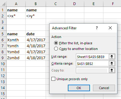
Create an additional table for the Advanced filter, entering your conditions in one line and giving each column the name of the corresponding column to filter – 'name' in our example. Type your criteria: <>x*, where '<>' means 'not equal to' and '*' allows matching any sequence of characters after 'x'. Thus, you will have 'does not begin with x' condition. Add other 5 of your own conditions, and apply advanced filter.
Hi. I can do an advanced filter using data on Sheet 1 and filter it onto Sheets 2-5 using different criteria for each time. However, I want the filters to automatically update when I add data to Sheet 1.
For example, I have data in cells A2:E28 on Sheet 1 and have filtered successfully onto the four sheets using different criteria each time. However, when I add a new row of data into A29:E29 on Sheet 1, I want this to automatically be filtered as per the advanced filters without having to reapply the filters each time.
Any help would be great. Thanks in advance.
Hi, David,
unfortunately, it's not possible.
As it is stated in the article: "Advanced Filter cannot be applied automatically since it has no pre-defined setup, it requires configuring the list range and criteria range manually."
I am looking a formula which can filter after satisfying the conditions..
I have 500 list of activities in column A, dates ( EX: 01-Jan-2017 to 31-Dec-2017 in format ) in Column B and in Column C ( Three different items like Complete, Pending, Ongoing etc)
Now I would like to extract out of 500 activities in column A , In January Month how many completed , How many pending & how many ongoing status in quantity.
Please can you help on this. Thanks for your support
Hi Naga,
You can try a Count if Function.
=Countif( Range(Month),”January”)
Or you can convert your data in to pivot table and easily you can count you data montly.
Hi I want to filter gps data from two columns (latitude,longitude)but I also need to filter them in order to have a range from 1 to 4 lets say is that possible? and how
Thanks
when i doing advance filtering, i got the the error message after clicking "ok" .."the extract range has a missing or invalid feild name".
please give me the solution.
Hi I need a formula that will track how many times a patient should been seen every 6 months (ex. Start date 1/1/2016 - ytd how many times was the patient seen?
hi,
you can use countifs function.