The tutorial shows how to write an IF OR statement in Excel to check for various "this OR that" conditions.
IF is one of the most popular Excel functions and very useful on its own. Combined with the logical functions such as AND, OR, and NOT, the IF function has even more value because it allows testing multiple conditions in desired combinations. In this tutorial, we will focus on using IF-and-OR formula in Excel.
IF OR statement in Excel
To evaluate two or more conditions and return one result if any of the conditions is TRUE, and another result if all the conditions are FALSE, embed the OR function in the logical test of IF:
In plain English, the formula's logic can be formulated as follows: If a cell is "this" OR "that", take one action, if not then do something else.
Here's is an example of the IF OR formula in the simplest form:
=IF(OR(B2="delivered", B2="paid"), "Closed", "Open")
What the formula says is this: If cell B2 contains "delivered" or "paid", mark the order as "Closed", otherwise "Open".
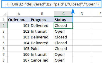
In case you want to return nothing if the logical test evaluates to FALSE, include an empty string ("") in the last argument:
=IF(OR(B2="delivered", B2="paid"), "Closed", "")
The same formula can also be written in a more compact form using an array constant:
=IF(OR(B2={"delivered","paid"}), "Closed", "")
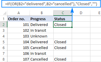
In case the last argument is omitted, the formula will display FALSE when none of the conditions is met.
Note. Please pay attention that an IF OR formula in Excel does not differentiate between lowercase and uppercase characters because the OR function is case-insensitive. In our case, "delivered", "Delivered", and "DELIVERED", are all deemed the same word. If you'd like to distinguish text case, wrap each argument of the OR function into EXACT as shown in this example.
Excel IF OR formula examples
Below you will find a few more examples of using Excel IF and OR functions together that will give you more ideas about what kind of logical tests you could run.
Formula 1. IF with multiple OR conditions
There is no specific limit to the number of OR conditions embedded into an IF formula as long as it is in compliance with the general limitations of Excel:
- In Excel 2007 and higher, up to 255 arguments are allowed, with a total length not exceeding 8,192 characters.
- In Excel 2003 and lower, you can use up to 30 arguments, and a total length shall not exceed 1,024 characters.
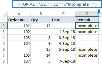
As an example, let's check columns A, B and C for blank cells, and return "Incomplete" if at least one of the 3 cells is blank. The task can be accomplished with the following IF OR function:
=IF(OR(A2="",B2="", C2=""),"Incomplete","")
And the result will look similar to this:
Formula 2. If a cell is this OR that, then calculate
Looking for a formula that can do something more complex than return a predefined text? Just nest another function or arithmetic equation in the value_if_true and/or value_if_false arguments of IF.
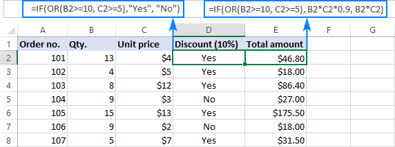
Say, you calculate the total amount for an order (Qty. multiplied by Unit price) and you want to apply the 10% discount if either of these conditions is met:
- in B2 is greater than or equal to 10, or
- Unit Price in C2 is greater than or equal to $5.
So, you use the OR function to check both conditions, and if the result is TRUE, decrease the total amount by 10% (B2*C2*0.9), otherwise return the full price (B2*C2):
=IF(OR(B2>=10, C2>=5), B2*C2*0.9, B2*C2)
Additionally, you could use the below formula to explicitly indicate the discounted orders:
=IF(OR(B2>=10, C2>=5),"Yes", "No")
The screenshot below shows both formulas in action:
Formula 3. Case-sensitive IF OR formula
As already mentioned, the Excel OR function is case-insensitive by nature. However, your data might be case-sensitive and so you'd want to run case-sensitive OR tests. In this case, perform each individual logical test inside the EXACT function and nest those functions into the OR statement.
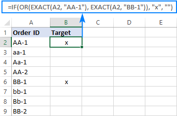
In this example, let's find and mark the order IDs "AA-1" and "BB-1":
=IF(OR(EXACT(A2, "AA-1"), EXACT(A2, "BB-1")), "x", "")
As the result, only two orders IDs where the letters are all capital are marked with "x"; similar IDs such as "aa-1" or "Bb-1" are not flagged:
Formula 4. Nested IF OR statements in Excel
In situations when you want to test a few sets of OR criteria and return different values depending on the results of those tests, write an individual IF formula for each set of "this OR that" criteria, and nest those IF's into each other.
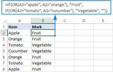
To demonstrate the concept, let's check the item names in column A and return "Fruit" for Apple or Orange and "Vegetable" for Tomato or Cucumber:
=IF(OR(A2="apple", A2="orange"), "Fruit", IF(OR(A2="tomato", A2="cucumber"), "Vegetable", ""))
For more information, please see Nested IF with OR/AND conditions.
Formula 5. IF AND OR statement
To evaluate various combinations of different conditions, you can do AND as well as OR logical tests within a single formula.
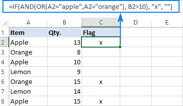
As an example, we are going to flag rows where the item in column A is either Apple or Orange and the quantity in column B is greater than 10:
=IF(AND(OR(A2="apple",A2="orange"), B2>10), "x", "")
For more information, please see Excel IF with multiple AND/OR conditions.
That's how you use IF and OR functions together. To have a closer look at the formulas discussed in this short tutorial, you are welcome to download our sample Excel IF OR workbook. I thank you for reading and hope to see you on our blog next week!
 by
by
218 comments
i used this and worked superb
=IFERROR(IF(FIND(AE2,AF2)=1,"PROCESS ON LINK","PROCESS ON LINK"),"PROCESS MISSING ON LINK")
PLANNE RING PROCESS Processes on the Link LINK CHECK
1000 1000,240,526,530,1000,240,526,530 PROCESS ON LINK
Look for the Planned ring Process Value in the Process on the Link and output Process ON LINK is found if not found print Process missing on Link
challenge was with multiple appearance hence the double process on Link, check for appearing once and then more than once as well and if not found if its error u out put the process missing on link
Hello Joel!
If I understand the question correctly, in order to count duplicate words within a text string, you need to split that text string into individual words. This can be done using the TEXTSPLIT function. Then use the SUMPRODUCT function to count the number of matches. The CHOOSE function will return the text based on the number of matches. Based on your information, the formula might look something like this:
=IFERROR(CHOOSE(SUMPRODUCT(--(TEXTSPLIT(AF2,,",")=(AE2&""))), "PROCESS ON LINK","Double","Triple"),"PROCESS MISSING ON LINK")
You can also use a combination of the SUMPRODUCT and LEN functions in Excel. Click here to read a detailed description of how to count words: Count specific words / text in a cell. Based on the information given, the formula could be as follows:
=IFERROR(CHOOSE(SUMPRODUCT((LEN(AF2)-LEN(SUBSTITUTE(AF2, AE2, "")))/LEN(AE2)), "PROCESS ON LINK","Double","Triple"),"PROCESS MISSING ON LINK")
I am building a property model which assumes an acquisition date and an escalation date. I want to use Nested if statements to build an income statement, which should incorporate the escalation of the income streams on the escalation dates. Please propose the formula to use.
Hi! Sorry, I do not fully understand the task. Give examples of source data and explain in detail what you want to do.
You can read more about nested IF formulas in this article: Nested IF in Excel – formula with multiple conditions, and also here: Excel Nested IF statements - examples, best practices and alternatives.
Hi need some support.
If cell v6 equal to 39 than 39 but is cell v6 is lower than 39 than need calculate v6-p5
Also is if cell v6 is 39 than ignore calculation in cell p5
Hi! I recommend reading this guide: Nested IF in Excel – formula with multiple conditions. Unfortunately I can't offer you a formula as your description is not very clear.
Also what need to do if i have calculation in cell p5 but want 0 if v6 is 39
I want to do this: if this, then this, or if this, then this, otherwise this
Example, if A2=Male, enter "man", of if A2 = Female, enter "woman", otherwise enter "unknown"
Hi Jim!
For multiple conditions, you can use nested IF function as described in this manual: Nested IF in Excel – formula with multiple conditions.
=IF(A2="Male","man",IF(A2="Female","woman","unknown"))
You can also use IFS function. You can find the examples and detailed instructions here: The new Excel IFS function instead of multiple IF.
=IFERROR(IFS(A2="Male","man",A2="Female","woman"),"unknown")
Hi there!
I am trying to assign dates to my parts when they will be completed biased on what step they are in.
a part has 9 different sequences it can be at and biased on what sequence it is at I can give an estimated date on when it will be completed.
IE
Part A is at sequence 50, it takes 5 days to complete it so it should be finished by 4-27-24.
I had this working for if OR statements for the first two locations but as soon as I added a third (and I need to add 9 different location total) i get an error saying there are to many arguments. Any ideas on what I can do? Below is what should work but I get the 'to many arguments error"
=IF(OR(E9="IPQA"), D8+H8, IF(OR(E9="PP1"), D8+I8), IF(OR(E9="PP2"), D8+j8), IF(OR(E9="MOLD"), D8+K8), IF(OR(E9="DEFLASH"), D8+L8), IF(OR(E9="ID"), D8+M8), IF(OR(E9="FINAL"), D8+N8), IF(OR(E9="FIN"), D8+O8))
Hi! You don't need to use the OR function for one condition. Also, your formula has a lot of unnecessary parentheses. To write nested IF functions correctly, use these guidelines: Nested IF in Excel – formula with multiple conditions. You can also find useful information in this article: Use the new Excel IFS function instead of nested IF.
Based on this information, the formula could be as follows:
=IF(E9="IPQA",D8+H8,IF(E9="PP1",D8+I8,IF(E9="PP2",D8+J8,IF(E9="MOLD",D8+K8,IF(E9="DEFLASH",D8+L8,IF(E9="ID",D8+M8,IF(E9="FINAL",D8+N8,IF(E9="FIN",D8+O8))))))))
Hello Sir,
1. I have a bunch of car names in cell B20 be like ( Civic,Jazz,BRV,CRV ,Figo,Endover,Ecosport,XL-6,Breeza,X-Presso,Xcross, Baleno, Thar,Bolero)
If B20 =any one value of (Civic,Jazz,BRV,CRV) then B21=Honda
if B20=any one value of (Figo,Endover,Ecosport) then B21=Ford
if B20=any one value of (XL-6,Breeza,X-Presso,Xcross, Baleno) then B21=Maruthi
if B20=any one value of (Thar,Bolero) then B21=Mahindra
I don't have the company names in my sheet so I need to compare the car name and give the car manufacturer detail in the next cell. Nearly i have 9000 so manually checing and updating is not possible. Please provide a query to accomplish it. Thanks in advance.
Hello! You must split the text in cell B20 by each name to search for car names. Then use the MATCH function to find matches in the Vehicle Name list (column K) and extract the corresponding manufacturer from the corresponding cell in column L using INDEX function.
=INDEX(L1:L10, INDEX(MATCH(TEXTSPLIT(B20,","),K1:K10,0), MATCH(TRUE,ISNUMBER(MATCH(TEXTSPLIT(B20,","),K1:K10,0)),0)))
I hope my advice will help you solve your task.
For more information, please visit: TEXTSPLIT function in Excel: split text strings by delimiter.
Is there any other command, shortcut , other method for the following query in excel.
=IF(OR(O2786="GITFASPRDSC1A",O2786="GITFASPRDSC10",O2786="GITBKPDEVSV01",O2786="GITBKPPRDSV01",O2786="GITFASPRDSC1B",O2786="GITNASPRDFS01",O2786="GITNASPRDFS02_DR",O2786="GITNASPRDFS03",O2786="GITNASSTGFS04_DR"),"GITFASPRDSC10")
Hi! I can't understand your formula and check it as I don't have your data. I can't guess what result you wanted to get.
I need help with generating a formula, please
If cell H birthday is between 6/3/20 - 9/1/20 cell I is equal to TE; if cell H birthday is between 9/2/19 - 6/2/20 cell I is equal to TK; if cell H birthday is between 9/2/18 - 9/1/19 cell I is equal to K
Hi! We have a special tutorial that can help to solve your problem: Excel IF between two numbers or dates. To use multiple time intervals in an IF formula, I recommend these instructions: Nested IF in Excel – formula with multiple conditions.
For example:
=IF(AND(A2>=DATEVALUE("6/3/20"), A2<=DATEVALUE("9/1/20")), "TE", IF(AND(A2>=DATEVALUE("9/2/19"), A2<=DATEVALUE("6/2/20")), "TK", ""))
If want to output as below, which formula should I used?
(98HVJM)HBRD2PT24KNOUV2PLG1K001H21 - Call
(OGEFJC)RA996TH3QTP1CSG8AS34000QRF - Call
(K0IHCC)IR6L50PF4HH077U6S3D80BK6UI - Call
(0004Ka)JWWB8A1VR1 - Email
else empty
Showed above in bracket will not change
Hi! Sorry, I have no idea exactly what the task is.
It's hard to tell exactly what you're asking for as it's currently written.
Currently I'm using like =IF(ISNUMBER(FIND("0004KaJ",A3)),"Email","Call")
It will always output Call in column,
wanted to have "" empty instead and only output when any of the above data input in A3
If I understand your task correctly, check cell A3 using the ISBLANK function. Read more: ISBLANK function in Excel to check if cell is blank.
=IF(ISBLANK(A3),"", IF(ISNUMBER(FIND("0004KaJ",A3)),"Email","Call"))
Hi, yes, it works, thanks alot
Column A has multiple ITEMS for eg - mango, banana, papaya, knife, spoons, garlic, ginger, tomato, potato, TV, Refrigerator, Microwave, Oven, Shirts, Pants, Shoes, Socks, Dell Laptop, Huawei Laptop, Lenovo Laptop, etc.
Now in Column B, Types Of Items must be grouped -
I need types of items =If(A1="mango","banana","papaya"),"FRUITS"),If( A1="knife", "spoons"),"Cutleries", if (A1="Garlic","potato","tomato,"Vegetables" and so on..
Hi! You can try a nested IF function as described in your question. For multiple conditions, I recommend using the IFS function. You can see other solutions for multiple conditions in this article: Excel Nested IF statements - examples, best practices and alternatives.
Example not correct for the Belgian version:
You have to use a ; between the statements in stead of '
I've read through so many examples and still getting an error in my formula.
I want to enter a value in a cell that depending on the range of that value then returns a specific price in another cell.
If value is 24 or less, return a price of $15.
If the value is between 25 and 34, return a price of $25
And so on.
How would you write this?
Hi! To describe conditions in an interval of numbers, take a look at the example in the first paragraph of this article: Excel Nested IF statement: examples, best practices and alternatives.
I have two column both contain tru,false and blank...I want my answer to return one if both column are true what formula do i use?
Hi! You can find the answer to your question in this article: IF AND in Excel: nested formula, multiple statements, and more. You can use the following formula to return 1 if both columns contain TRUE, and return 0 otherwise:
=IF(AND(A1=TRUE, B1=TRUE), 1, 0)
Thank you. I figured it out based on that article and wrote the following statement:
=IF(C2>54,55, IF(C2>=45,45, IF(C2>=35,35, IF(C2>=25,25, IF(C2>=1,15)))))
Now I need to add another test. If the value in B2 = No, then it's one set of pricing based on a range (as shown above), but if the value in B2 = Yes, then the pricing is different.
Hi! If I understand your task correctly, try the following formula:
=IF(B2="Yes", IF(C2>54,55, IF(C2>=45,45, IF(C2>=35,35, IF(C2>=25,25, IF(C2>=1,15))))), ..different pricing........ )
There are detailed instructions in the article I've already recommended to you.
how to write if condition in excel in a cell either for addition or subtraction or multiplication?
For eg.:
Customer Purchased Item ₹ 6,989 ₹ 6,989 ₹ 6,989
Customer Purchased Item ₹ 40,000 ₹ 46,989 ₹ 46,989
Customer Purchased Item ₹ 28,541 ₹ 75,530 ₹ 75,530
Cash Received from customer ₹ 35,000 ₹ 40,530 ₹ 40,530
Customer paid chq #: 39759 ₹ 39,759 ₹ 771 ₹ 771
No one will be able to guess what you want to do with your data. To learn how to write an IF condition, see the recommendations in the comment above.
how to write if condition in excel in a cell either for addition or subtraction or multiplication?
Hi Jeevan,
if you would like to write a if condition in excel that either for addition or subtraction or multiplication, you must be prepare with the logic what you want to write.
Hi! I recommend reading the article above carefully. Also this article will be useful: IF function in Excel: formula examples for text, numbers, dates, blanks.
Hello. I have a construction bid spreadsheet that incorporates a tiering labor cost, dependent upon the square footage of material. Example: 1-30sf is $225 in labor, 31-59sf is $337.50, 60sf+ is $450. My working formula to calculate the material cost and labor is below:
=IFS(B24=60,SUM(C$14*B24)+SUM(C$15*B24)+C$18,B24>=31,SUM(C$14*B24)+SUM(C$15*B24)+C$17,B24>=1,SUM(C$14*B24)+SUM(C$15*B24)+C$16)
I am now adding a flat labor rate to install the material in a specific pattern. This flat rate would override the tiering labor rates above if using the pattern. My thought is to add a "yes"/"no" dropdown in cell D21 to select if the material will be installed in a pattern, with the flat labor rate in C21. The square footage of the job in in cell B24 of the formula below.
What formula would I use to use the above formula if D21 is "NO", but if D21 is "YES" use a different formula such as B24=SUM(C$14*B24)+SUM(C$15*B24)+C21?
I continue to get errors...
Hi! Use the IF function to do calculations depending on the value of B21:
=IF(B21="Yes", SUM(C$14*B24)+SUM(C$15*B24)+C21, IFS(B24=60,SUM(C$14*B24)+SUM(C$15*B24)+C$18,B24>=31, SUM(C$14*B24)+SUM(C$15*B24)+C$17,B24>=1, SUM(C$14*B24)+SUM(C$15*B24)+C$16))
Hope this is what you need.
Hi,
I need one formula but not able to figure out how to apply. I have two cells. in cell 1 entries may be(Yes, No) in cell 2 entries may be (Required, Not required), now the conditions I want to check. if in cell 1 "Yes" and Cell 2 "Required" then output should be "Yes". But if in cell 1 "Yes" and in Cell 2 "Not Required" then the answer should be "No".
Hi! The following tutorial should help: Excel IF statement with multiple conditions. For example:
=IF(AND(A1="yes",A2="required"),"yes", IF(AND(A1="yes",A2="not required"),"no",""))
Need a formula for the following....I am beating my brains out
This is what I've tried by it isn't working.
=IF(AND(SUM(H30+J30)=2,"1"),SUM(H30+J30)>3,"2")
My objective is....
If the sum of H30+J30=2 I want the cell to return "1", and If the sum of H30+J30 is >= 4 I want the cell to return "2" but if the sum of H30+J30=3 I want it to return 0.
Can anyone help me???
Hi! You can find the examples and detailed instructions here: Excel Nested IF statement: examples, best practices and alternatives. For example:
=IF(SUM(H30+J30)=2,"1", IF(SUM(H30+J30)>3,"2",""))
In Colum H I have a weekly cost 398.70
in Column I - I want to be able to put in a "Y" or an "N".
I want the Y to be half the amount of 397.70 (meaning apportioned 1:2 so it would be 199.35)
I want the N to be 398.70 (meaning the full amount not apportioned)
Hi! Unfortunately, it is not clear which cells you want to compare. Column I cannot contain a number and text at the same time. I recommend reading this guide: IF function in Excel: formula examples for text, numbers, dates, blanks.
Hi there, im trying to give a single cell a number value based off 2 words. Ive tried the IF but cant seem seem to figure it out. I want
Cell F3 to give a number 2 if its a "W" and cell F3 also to give me a -1 if the text is a "L". Ive done IF(f3="w",2) and it works but cant figure out to add the "L" portion to the formula
Hey, so I am having troubling writing an if statement. I tried using concrate with it also so I can reflect two different outcomes. But everytime I create a formula it only reflects one option of what I wanted.
For example I was using :
=if(or(e1=“sw turnstile in”,”se lby turnstile in”, “in”,”out”),if(or(e1=“sw turnstile out”,”se turnstile out”,”out”,”in”)))