The tutorial shows how to use IFERROR in Excel to catch errors and replace them with a blank cell, another value or a custom message. You will learn how to use the IFERROR function with Vlookup and Index Match, and how it compares to IF ISERROR and IFNA.
"Give me the place to stand, and I shall move the earth," Archimedes once said. "Give me a formula, and I shall make it return an error," an Excel user would say. In this tutorial, we won't be looking at how to return errors in Excel, we'd rather learn how to prevent them in order to keep your worksheets clean and your formulas transparent.
Excel IFERROR function - syntax and basic uses
The IFERROR function in Excel is designed to trap and manage errors in formulas and calculations. More specifically, IFERROR checks a formula, and if it evaluates to an error, returns another value you specify; otherwise, returns the result of the formula.
The syntax of the Excel IFERROR function is as follows:
Where:
- Value (required) - what to check for errors. It can be a formula, expression, value, or cell reference.
- Value_if_error (required) - what to return if an error is found. It can be an empty string (blank cell), text message, numeric value, another formula or calculation.
For example, when dividing two columns of numbers, you may get a bunch of different errors if one of the columns contains empty cells, zeros or text.
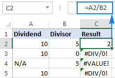
To prevent that from happening, use the IFERROR function to catch and handle errors the way you want.
If error, then blank
Supply an empty string (") to the value_if_error argument to return a blank cell if an error is found:
=IFERROR(A2/B2, "")
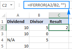
If error, then show a message
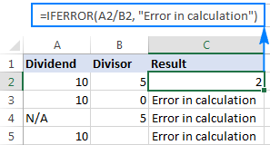
You can also display your own message instead of Excel's standard error notation:
=IFERROR(A2/B2, "Error in calculation")
5 things you should know about Excel IFERROR function
- The IFERROR function in Excel handles all error types including #DIV/0!, #N/A, #NAME?, #NULL!, #NUM!, #REF!, and #VALUE!.
- Depending on the contents of the value_if_error argument, IFERROR can replace errors with your custom text message, number, date or logical value, the result of another formula, or an empty string (blank cell).
- If the value argument is a blank cell, it is treated as an empty string (''') but not an error.
- IFERROR was introduced in Excel 2007 and is available in all subsequent versions of Excel 2010, Excel 2013, Excel 2016, Excel 2019, Excel 2021, and Excel 365.
- To trap errors in Excel 2003 and earlier versions, use the ISERROR function in combination with IF, as shown in this example.
IFERROR formula examples
The following examples show how to use IFERROR in Excel in combination with other functions to accomplish more complex tasks.
Excel IFERROR with Vlookup
One of the most common uses of the IFERROR function is telling the users that the value they are searching for does not exist in the data set. For this, you wrap a VLOOKUP formula in IFERROR like this:
If the lookup value is not in the table you are looking in, a regular Vlookup formula would return the #N/A error:

For your users' piece of mind, wrap VLOOKUP in IFERROR and display a more informative and user-friendly message:
=IFERROR(VLOOKUP(A2, 'Lookup table'!$A$2:$B$4, 2,FALSE), "Not found")
The screenshot below shows this Iferror formula in Excel:

If you'd like to trap only #N/A errors but not all errors, use the IFNA function instead of IFERROR.
For more Excel IFERROR VLOOKUP formula examples, please check out these tutorials:
Nested IFERROR functions to do sequential Vlookups in Excel
In situations when you need to perform multiple Vlookups based on whether the previous Vlookup succeeded or failed, you can nest two or more IFERROR functions one into another.
Supposing you have a number of sales reports from regional branches of your company, and you want to get an amount for a certain order ID. With A2 as the lookup value in the current sheet, and A2:B5 as the lookup range in 3 lookup sheets (Report 1, Report 2 and Report 3), the formula goes as follows:
=IFERROR(VLOOKUP(A2,'Report 1'!A2:B5,2,0),IFERROR(VLOOKUP(A2,'Report 2'!A2:B5,2,0),IFERROR(VLOOKUP(A2,'Report 3'!A2:B5,2,0),"not found")))
The result will look something similar to this:

For the detailed explanation of the formula's logic, please see How to do sequential Vlookups in Excel.
IFERROR in array formulas
As you probably know, array formulas in Excel are meant to perform multiple calculations within a single formula. If you supply an array formula or expression that results in an array in the value argument of the IFERROR function, it'd return an array of values for each cell in the specified range. The below example shows the details.
Let's say, you have Total in column B and Price in column C, and you want to calculate Total Quantity. This can be done by using the following array formula, which divides each cell in the range B2:B4 by the corresponding cell of the range C2:C4, and then adds up the results:
=SUM($B$2:$B$4/$C$2:$C$4)
The formula works fine as long as the divisor range does not have zeros or empty cells. If there is at least one 0 value or blank cell, the #DIV/0! error is returned:
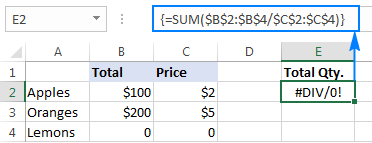
To fix that error, simply do the division within the IFERROR function:
=SUM(IFERROR($B$2:$B$4/$C$2:$C$4,0))
What the formula does is to divide a value in column B by a value in column C in each row (100/2, 200/5 and 0/0) and return the array of results {50; 40; #DIV/0!}. The IFERROR function catches all #DIV/0! errors and replaces them with zeros. And then, the SUM function adds up the values in the resulting array {50; 40; 0} and outputs the final result (50+40=90).

Note. Please remember that array formulas should be completed by pressing the Ctrl + Shift + Enter shortcut.
IFERROR vs. IF ISERROR
Now that you know how easy it is to use the IFERROR function in Excel, you may wonder why some people still lean towards using the IF ISERROR combination. Does it have any advantages compared to IFERROR? None. In the bad old days of Excel 2003 and lower when IFERROR did not exist, IF ISERROR was the only possible way to trap errors. In Excel 2007 and later, it's just a bit more complex way to achieve the same result.
For instance, to catch Vlookup errors, you can use either of the below formulas.
In Excel 2007 - Excel 2016:
In all Excel versions:
Notice that in the IF ISERROR VLOOKUP formula, you have to Vlookup twice. In plain English, the formula can be read as follows: If Vlookup results in error, return "Not found", otherwise output the Vlookup result.
And here is a real-life example of an Excel If Iserror Vlookup formula:
=IF(ISERROR(VLOOKUP(D2, A2:B5,2,FALSE)),"Not found", VLOOKUP(D2, A2:B5,2,FALSE ))

For more information, please see Using ISERROR function in Excel.
IFERROR vs. IFNA
Introduced with Excel 2013, IFNA is one more function to check a formula for errors. Its syntax is similar to that of IFERROR:
In what way is IFNA different from IFERROR? The IFNA function catches only #N/A errors while IFERROR handles all error types.
In which situations you may want to use IFNA? When it is unwise to disguise all errors. For example, when working with important or sensitive data, you may want to be alerted about possible faults in your data set, and standard Excel error messages with the "#" symbol could be vivid visual indicators.
Let's see how you can make a formula that displays the "Not found" message instead of the N/A error, which appears when the lookup value is not present in the data set, but brings other Excel errors to your attention.
Supposing you want to pull Qty. from the lookup table to the summary table as shown in the screenshot below. Using the Excel Iferror Vlookup formula would produce an aesthetically pleasing result, which is technically incorrect because Lemons do exist in the lookup table:
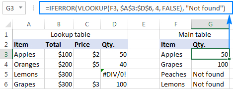
To catch #N/A but display the #DIV/0 error, use the IFNA function in Excel 2013 and Excel 2016:
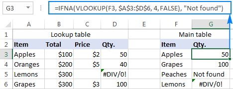
=IFNA(VLOOKUP(F3,$A$3:$D$6,4,FALSE), "Not found")
Or, the IF ISNA combination in Excel 2010 and earlier versions:
=IF(ISNA(VLOOKUP(F3,$A$3:$D$6,4,FALSE)),"Not found", VLOOKUP(F3,$A$3:$D$6,4,FALSE))
The syntax of the IFNA VLOOKUP and IF ISNA VLOOKUP formulas are similar to that of IFERROR VLOOKUP and IF ISERROR VLOOKUP discussed earlier.
As shown in the screenshot below, the Ifna Vlookup formula returns "Not found" only for the item that is not present in the lookup table (Peaches). For Lemons, it shows #DIV/0! indicating that our lookup table contains a divide by zero error:
For more details, please see Using IFNA function in Excel.
Best practices for using IFERROR in Excel
By now you already know that the IFERROR function is the easiest way to catch errors in Excel and mask them with blank cells, zero values, or custom messages of your own. However, that does not mean you should wrap each and every formula with error handling. The following simple recommendations may help you keep the balance.
- Don't trap errors without a reason.
- Wrap the smallest possible part of a formula in IFERROR.
- To handle only specific errors, use an error handling function with a smaller scope:
- IFNA or IF ISNA to catch only #N/A errors.
- ISERR to catch all errors except for #N/A.
This is how you use the IFERROR function in Excel to trap and handle errors. To have a closer look at the formulas discussed in this tutorial, you are welcome to download our sample IFERROR Excel workbook. I thank you for reading and hope to see you on our blog next week.
 by
by
40 comments
made latest excel ,
but its not working older version, need your support
=IFERROR(IF(B$3>$N5,CONCATENATE(B$4,B$5+$N5,".",SEQUENCE(8,1,0,1)),""),"")
Hi! The SEQUENCE function is only supported in Excel 365, Excel 2021, and Excel for the web.
Hi What does this means?
=IFERROR(ROUND(AVERAGE(INDIRECT($D6 & $E$4 & F$4):INDIRECT($D6 & $E$4 & F$5)),1),0)
Hi! If you wrote this formula, you must have an idea of what your goal is. You can learn more about INDIRECT function in Excel in this article on our blog: Excel INDIRECT function - basic uses and formula examples.
I have a simple IFERROR formula to calculate a variance% between actuals and budget. Currently, the variance% is showing as a negative value despite actuals outperforming budget.
Example:
Net Income: ($20,000)
Budgeted Net Income: ($30,000)
Variance: +$10,000
Variance%: -33%
*Current formula: =IFERROR(Variance/Budget,"-") results in a negative %. How can I get this to calculate the variance% to be determined by the positive value of the variance amount instead of the mathematical result?
Hi! Your formula and the data you wrote cannot give a negative percent result. 10000/30000=33%. However, you can always apply the ABS function to use the absolute value of the variance.
If I use the ABS function, it will always return a positive result. Correct? I want it to return a negative result when applicable.
I understand from your question that you always want a positive result. I think these instructions will help: How to calculate percentage in Excel - formula examples.
No, I want the sign of the variance% to be determined by the variance amount. If the variance amount is a positive number, I want the variance% to be positive. If the variance amount is negative, I want the variance% to be negative.
In the article I recommended to you, read the paragraph - How to calculate percent difference in Excel.
Hi all, I am looking for a MATCH formula for the following.
SHEET 1: I type a Home# (example Home-1) in column A and a stage (example DRYWALL) in Column B.
Sheet 2: I type a home number again is Column A I would like column B to pull automatically from Sheet one Column B. But it has to match that specific home number.
Reference, I have multiple homes and throughout multiple spreadsheets I update the specific home #’s stage and would like to just update it on sheet 1 and it auto pull onto multiple different sheets.
Hello! You can extract the required value with the VLOOKUP function following these guidelines: Excel VLOOKUP function tutorial with formula examples.
You can also use INDEX+MATCH as described in these instructions: Excel INDEX MATCH vs. VLOOKUP - formula examples.
Hi all,
Does anyone know a formula so it can highlight if a date has changed? I have 2 columns of dates which have hundreds of rows completed and I need a formula to highlight if one of the dates have changed from one column to another. I can then drag this down the rows. My end goal is to give a percentage of dates that have changed
Hi! If I understand your task correctly, this article may be helpful: Compare two columns for matches and differences.
I cannot tell you how helpful this has been. Thank you very much :-)
Hi!
I am comparing the values in two different columns. If the value from column B exists in column A, I want it to say "OLD", but if the value in column B does not exist in column A, I want it to say "NEW". I got it to say "NEW", but for "OLD, it's returning the same name again. How can I customize this second part?
=IFERROR(VLOOKUP(C2,$A$2:$A$1000,1,FALSE),"NEW")
Thank you
Hi! Use the IF function to get "OLD" if VLOOKUP returns a cell value, and get "NEW" if VLOOKUP returns an error.
=IF(ISERROR(VLOOKUP(C2,$A$2:$A$1000,1,FALSE)),"NEW","OLD")
Hi, I'm working on a time-sheet of sorts with a 24 hour format. Typical in-times will be 18:00 and out-times will be 6:00. I'm using the following formula to calculate the total hours worked:
In time Out Time Total Hours
18:00 6:00 =IF((F26-E26)>0,F26-E26,IF((F26-E26)<0,-(F26-E26),IF((F26-E26=0),0)))
However, if the person is on leave, we will write text on the in-time cell resulting in a #VALUE! error for the total hours worked. I would like to have a zero replace the error value. What do you recommend? Thank you for any help with this!
Hi! To replace the error message with another value, use the IFERROR function.
Try this formula:
=IFERROR(IF((F26-E26)>0,F26-E26,IF((F26-E26)<0,-(F26-E26),IF((F26-E26=0),0))),0)
I need a formula for this situation, i have many cells fill with same data but when i change data in any cell then i want those changes with cell reference in my reporting cell
for example
cell A1 sunday cell B1 sunday cell C1 sunday cell D1 sunday cell E1 sunday cell F1 sunday but if i change Cell E1 monday
then my reporting cell A2 may be show "E1 Monday" otherwise reporting cell A2 may shows "no changes"
sir please help me to create this formula
thank you
Hi!
Excel formula cannot detect a change in a value in a cell. An Excel formula can compare a value in a cell to a predefined number or text string. You can use the IF function to show the result of a value comparison.
I have the following formula:
=IFERROR(@INDEX('Data Sheet'!$BB$2:$BD$2,1,COUNTIF('Data Sheet'!$BB$2:$BD$6,B32))," ")
of which I only need it to be actioned if the outcome of that same formula is not equal to a certain value.. How can i do that?
Hi!
For conditional calculations, try to use IF function:
IF([formula]=[value],"",[formula])
Hello, i have a worksheet which has a formula referencing to calculating a discounted price, =F9*(1-H9). I have rows that do not have any price or % present resulting in my calucation giving me the #VALUE! error when i drag the formula down. is there any way i can use the IFERROR? i have tried a few different ways but i cannot get it to work. I do not want to hide as there are totals at the end of the rows which also give the same error. thanks for any help
Hello!
Instructions and examples of using IFERROR can be found in this article above.
For example,
=IFERROR(F9*(1-H9),0)
Hi there,
It is great you can lean on real pros in the field.
Trying to figure out solution for the following problem.
1. Replacing the consecutives appearances of #N/A value in a column with dynamically incremental values for each appearance of #N/A down the column starting with particular number.
For example:
1st #N/A appearance to be replaced with 10000
2nd #N/A appearance to be replaced with 10001 and so on.
To a moment all the #N/A appearances in the column of the data are replaced with those consecutive numbers.
I know I am close, but I am missing something.
Thanks in advance
Svetlozar Todorov
Hello!
Maybe this formula will work for you.
=IFNA(VLOOKUP(F2,$A$3:$B$13,2,FALSE), COUNTIF($D$2:D2,">9999")+10000)
It is assumed that it is written in cell D3
=IFNA(VLOOKUP(F2,$A$3:$B$13,2,FALSE),COUNTIF($D$2:D2,">9999")+10000)
Hello!
If the first table is A3:A13 and the second table is D3:D13 then try the formula in cell E3
=IFERROR(VLOOKUP(D3,$A$3:$B$13,2,FALSE),MAX(MAX($B$3:$B$13)+1,MAX($E$2:E2)+1))
Сopy it down along the column
I need formula, to extract only 3 columns to separate sheet
Considering Product type located in Q column, it has to get Column D Assest ID & Price which in T column into new sheet.
Everything to be extract with formula only from Main sheet
Hi Alexander,
I have edited the formula, while I was trying to figure your logic out.
What is the point of a range A:B? I have edited to A:A,
Same for the second part :
MAX(MAX($B$3:$B$13) - That was edited to A:A and the next part
"MAX($E$2:E2)+1))" - is this correct the formula is column E. What is this part serving, as the formula is supposed to be filled in this column.
The result of different edits is not populating incremental values for the missing CodeID, but is pasting the same value which is the highest in the column + 1.
Appreciate the efforts!
Thanks!
Svetlozar Todorov
(Table 1)
Start Page | End Page
1 3
4 5
6 26
27 27
28 28
29 29
30 32
(Table 2)
Start Page | End Page
1 3
4 5
6 6
7 26
27 27
28 29
29 29
30 32
How to Compare Two table use formula?
I expect result for below
Table 1 Table 2
1 3 1 3
4 5 4 5
6 7 6 26
8 26 Error
27 27 27 27
28 28 28 29 Error
29 29 29 29
30 32 30 32
Hi!
I recommend reading this guide: How to compare two Excel files or sheets for differences.
I am trying to do a simple add and average of a column that is in percentage format. For example:
Column
50%
100%
50%
80%
Average Score: 70%
I keep getting a DIV 0 error
Hi!
Your error means division by zero. What formula are you using?
=IFERROR(MATCH(E10,item_ID,0)+2,'''') The above formula is showing a error message in my Excel 2016. That formula is correct and it worked in another PC which having Excel 2013. Please help me to get rid of this error.
Hello!
Your formula has a reference to the named range item_ID. I think your file does not have it. Create a named range item_ID in the desired cells.
I have a formula that is working, but it is not giving me a true picture.
This is the current cell(B5) formula: =IFERROR(IF(AND(AA5="",AJ5=""),"",$A$2-$AJ5),"")
I need this cell(B5) to be BLANK if the adjacent cell(C5) is populated. C5 has a formula in it that gives me a number or a BLANK.
Hello David!
If I understand your task correctly, the following formula should work for you:
=IF(C5<>"",IFERROR(IF(AND(AA5="",AJ5=""),"",$A$2-$AJ5),""),"")
I hope this will help
A1 1
A2 2
A3 ERROR
A4 4
if we do sum(A1:A4), sum should'nt work, its there any way
Please suggest
Hello Munawar!
The value in Cell A3 has been received as a result of the incorrect performance of some formula. It is impossible to use this cell with an error in Excel formulas.
To avoid such situations, it is necessary to use the IFERROR function.
To learn more about it, please read this article on our blog: https://www.ablebits.com/office-addins-blog/excel-iferror-function-formula-examples/
You can also see examples of the IFERROR function usage there. Undoubtedly, they will be helpful to you.