In this quick lesson, you will learn how to filter in Excel dynamically with formulas. Examples to filter duplicates, cells containing certain text, with multiple criteria, and more.
How do you usually filter in Excel? For the most part, by using Auto Filter, and in more complex scenarios with Advanced Filter. Being fast and powerful, these methods have one significant drawback - they do not update automatically when your data changes, meaning you would have to clean up and filter again. The introduction of the FILTER function in Excel 365 becomes a long-awaited alternative to the conventional features. Unlike them, Excel formulas recalculate automatically with each worksheet change, so you'll need to set up your filter just once!
Excel FILTER function
The FILTER function in Excel is used to filter a range of data based on the criteria that you specify.
The function belongs to the category of Dynamic Arrays functions. The result is an array of values that automatically spills into a range of cells, starting from the cell where you enter a formula.
The syntax of the FILTER function is as follows:
Where:
- Array (required) - the range or array of values that you want to filter.
- Include (required) - the criteria supplied as a Boolean array (TRUE and FALSE values).
Its height (when data is in columns) or width (when data is in rows) must be equal to the that of the array argument. - If_empty (optional) - the value to return when no entries meet the criteria.
The FILTER function is only available in Excel for Microsoft 365 and Excel 2021. In Excel 2019, Excel 2016 and earlier versions, it is not supported.
Basic Excel FILTER formula
For starters, let's discuss a couple of very simple cases just to gain more understanding how an Excel formula to filter data works.
From the below data set, supposing you want to extract the records with a specific value in the Group, column, say group C. To have it done, we supply the expression B2:B13="C" to the include argument, which will produce a required Boolean array, with TRUE corresponding to "C" values.
=FILTER(A2:C13, B2:B13="C", "No results")
In practice, it's more convenient to input the criteria in a separate cell, e.g. F1, and use a cell reference instead of hardcoding the value directly in the formula:
=FILTER(A2:C13, B2:B13=F1, "No results")
Unlike Excel's Filter feature, the function does not make any changes to the original data. It extracts the filtered records into the so-called spill range (E4:G7 in the screenshot below), beginning in the cell where the formula is entered:
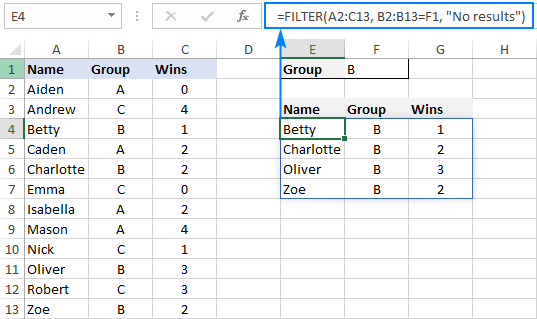
If no records match the specified criteria, the formula returns the value you put in the if_empty argument, "No results" in this example:
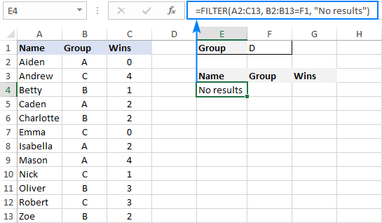
If you'd rather return nothing in this case, then supply an empty string ("") for the last argument:
=FILTER(A2:C13, B2:B13=F1, "")
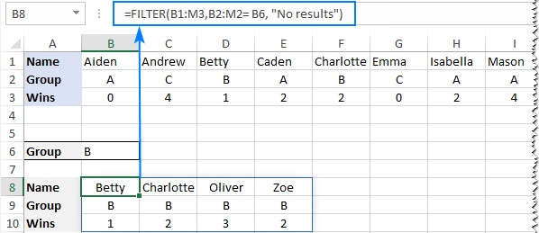
In case your data is organized horizontally from left to right like shown in the screenshot below, the FILTER function will work nicely too. Just make sure you define appropriate ranges for the array and include arguments, so that the source array and Boolean array have the same width:
=FILTER(B2:M4, B3:M3= B7, "No results")
Excel FILTER function - usage notes
To effectively filter in Excel with formulas, here are a couple of important points to take notice of:
- The FILTER function automatically spills the results vertically or horizontally in the worksheet, depending on how your original data is organized. So, please make sure you always have enough empty cells down and to the right, otherwise you'll get a #SPILL error.
- The results of the Excel FILTER function are dynamic, meaning they update automatically when values in the original data set change. However, the range supplied for the array argument is not updated when new entries are added to the source data. If you wish the array to resize automatically, then convert it to an Excel table and build formulas with structured references, or create a dynamic named range.
How to filter in Excel - formula examples
Now that you know how a basic Excel filter formula works, it's time to get some insights into how it could be extended for solving more complex tasks.
Filter with multiple criteria (AND logic)
To filter data with multiple criteria, you supply two or more logical expressions for the include argument:
The multiplication operation processes the arrays with the AND logic, ensuring that only the records that meet all the criteria are returned. Technically, it works this way:
The result of each logical expression is an array of Boolean values, where TRUE equates to 1 and FALSE to 0. Then, the elements of all the arrays in the same positions are multiplied. Since multiplying by zero always gives zero, only the items for which all the criteria are TRUE get into the resulting array, and consequently only those items are extracted.
The below examples show this generic formula in action.
Example 1. Filter multiple columns in Excel
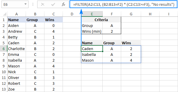
Extending our basic Excel FILTER formula a little further, let's filter the data by two columns: Group (column B) and Wins (column C).
For this, we set up the following criteria: type the name of the target group in F2 (criteria1) and the minimum required number of wins in F3 (criteria2).
Given that our source data is in A2:C13 (array), groups are in B2:B13 (range1) and wins are in C2:C13 (range2), the formula takes this form:
=FILTER(A2:C13, (B2:B13=F2) * (C2:C13>=F3), "No results")
As the result, you get a list of players in group A who have secured 2 or more wins:
Example 2. Filter data between dates
First off, it should be noted that it's not possible to make up a generic formula to filter by date in Excel. In different situations, you will need to build criteria differently, depending on whether you want to filter by a specific date, by month, or by year. The purpose of this example is to demonstrate the general approach.
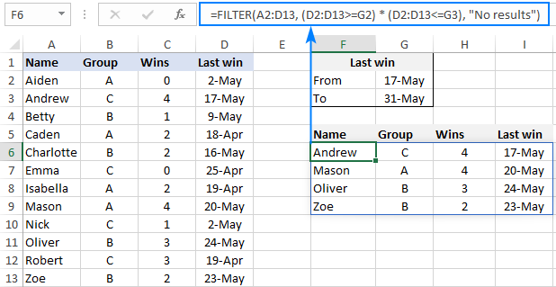
To our sample data, we add one more column containing the dates of the last win (column D). And now, we will extract the wins that occurred in a specific period, say between May 17 and May 31.
Please notice that in this case, both criteria apply to the same range:
=FILTER(A2:D13, (D2:D13>=G2) * (D2:D13<=G3), "No results")
Where G2 and G3 are the dates to filter between.
Filter with multiple criteria (OR logic)
To extract data based on multiple OR condition, you also use logical expressions like shown in the previous examples, but instead of multiplying, you add them up. When the Boolean arrays returned by the expressions are summed, the resulting array will have 0 for entries that do not meet any criteria (i.e. all the criteria are FALSE), and such entries will be filtered out. The entries for which at least one criterion is TRUE will be extracted.
Here's the generic formula to filter columns with the OR logic:
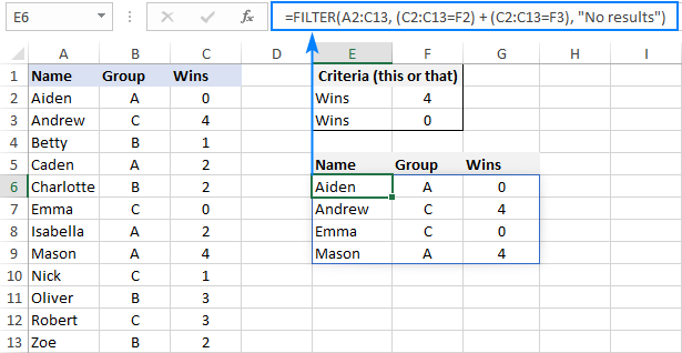
As an example, let's extract a list of players that have this or that number of wins.
Assuming the source data is in A2:C13, wins are in C2:C13, and the win numbers of interest are in F2 and F3, the formula would go as follows:
=FILTER(A2:C13, (C2:C13=F2) + (C2:C13=F3), "No results")
As the result, you know which players have won all the games (4) and which have won none (0):
Filter based on multiple AND as well as OR criteria
In situation when you need to apply both criteria types, remember this simple rule: join the AND criteria with asterisk (*) and OR criteria with the plus sign (+).
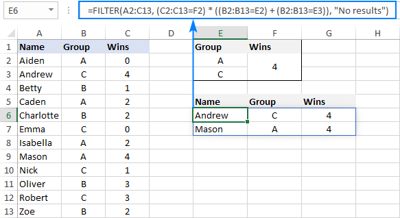
For example, to return a list of players that have a given number of wins (F2) AND belong to the group mentioned in either E2 OR E3, build the following chain of logical expressions:
=FILTER(A2:C13, (C2:C13=F2) * ((B2:B13=E2) + (B2:B13=E3)), "No results")
And you will get the following result:
How to filter duplicates in Excel
When working with huge worksheets or combining data from different sources, there's often a possibility that some duplicates would sneak in.
If you are looking to filter out duplicates and extract unique items, then use the UNIQUE function as explained in the above linked tutorial.
If your goal is to filter duplicates, i.e. extract entries that occur more than once, then use the FILTER function together with COUNTIFS.
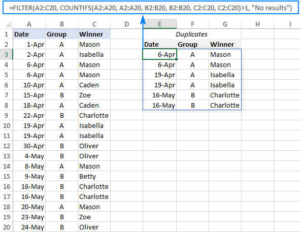
The idea is to get the occurrences counts for all the records and extract those greater than 1. To get the counts, you supply the same range for each criteria_range / criteria pair of COUNTIFS like this:
For example, to filter duplicate rows from the data in A2:C20 based on the values in all 3 columns, here's the formula to use:
=FILTER(A2:C20, COUNTIFS(A2:A20, A2:A20, B2:B20, B2:B20, C2:C20, C2:C20)>1, "No results")
Tip. To filter duplicates based on the values in the key columns, include only those specific columns in the COUNTIFS function.
How to filter out blanks in Excel
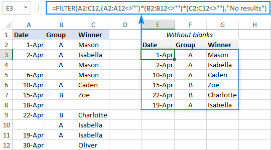
A formula for filtering out blank cells is, in fact, a variation of the Excel FILTER formula with multiple AND criteria. In this case, we check whether all (or particular) columns have any data in them and exclude the rows where at least one cell is empty. To identify non-blank cells, you use the "not equal to" operator (<>) together with an empty string ("") like this:
With the source data in A2:C12, to filter out rows containing one or more blank cells, the following formula is entered in E3:
Filter cells containing specific text
To extract cells that contain certain text, you can use the FILTER function together with the classic If cell contains formula:
Here's how it works:
- The SEARCH function looks for a specified text string in a given range and returns either a number (the position of the first character) or #VALUE! error (text not found).
- The ISNUMBER function converts all the numbers to TRUE and errors to FALSE and passes the resulting Boolean array to the include argument of the FILTER function.
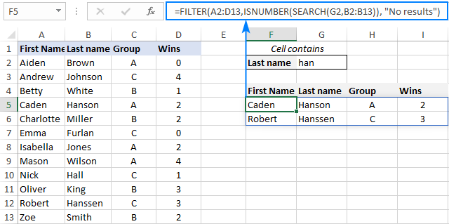
For this example, we've added the Last names of players in B2:B13, typed the part of the name we want to find in G2, and then use the following formula to filter the data:
=FILTER(A2:D13, ISNUMBER(SEARCH(G2, B2:B13)), "No results")
As the result, the formula retrieves the two surnames containing "han":
Filter and calculate (Sum, Average, Min, Max, etc.)
A cool thing about the Excel FILTER function is that it can not only extract values with conditions, but also summarize the filtered data. For this, combine FILTER with aggregation functions such as SUM, AVERAGE, COUNT, MAX or MIN.
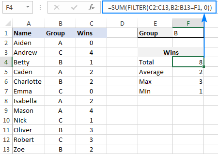
For instance, to aggregate data for a specific group in F1, use the following formulas:
Total wins:
=SUM(FILTER(C2:C13, B2:B13=F1, 0))
Average wins:
=AVERAGE(FILTER(C2:C13, B2:B13=F1, 0))
Maximum wins:
=MAX(FILTER(C2:C13, B2:B13=F1, 0))
Minimum wins:
=MIN(FILTER(C2:C13, B2:B13=F1, 0))
Please pay attention that, in all the formulas, we use zero for the if_empty argument, so the formulas would return 0 if no values meeting the criteria are found. Supplying any text such as “No results” would result in a #VALUE error, which is obviously the last thing you want :)
Case-sensitive FILTER formula
A standard Excel FILTER formula is case-insensitive, meaning it makes no distinction between lowercase and uppercase characters. To distinguish text case, nest the EXACT function in the include argument. This will force FILTER to do logical test in a case-sensitive manner:
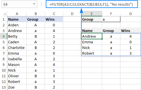
Supposing, you have both groups A and a and wish to extract records where the group is the lowercase "a". To have it done, use the following formula, where A2:C13 is the source data and B2:B13 are groups to filter:
=FILTER(A2:C13, EXACT(B2:B13, "a"), "No results")
As usual, you can input the target group in a predefined cell, say F1, and use that cell reference instead of hardcoded text:
=FILTER(A2:C13, EXACT(B2:B13, F1), "No results")
How to FILTER data and return only specific columns
For the most part, filtering all columns with a single formula is what Excel users want. But if your source table contains tens or even hundreds of columns, you may certainly want to limit the results to a few most important ones.
Example 1. Filter some adjacent columns
In situation when you want some neighboring columns to appear in a FILTER result, include only those columns in array because it is this argument that determines which columns to return.
In the basic FILTER formula example, supposing you wish to return the first 2 columns (Name and Group). So, you supply A2:B13 for the array argument:
=FILTER(A2:B13, B2:B13=F1, "No results")
As the result, we get a list of participants of the target group defined in F1:

Example 2. Filter non-adjacent columns
To cause the FILTER function to return non-contiguous columns, use this clever trick:
- Make a FILTER formula with the desired condition(s) using the entire table for array.
- Nest the above formula inside another FILTER function. To configure the "wrapper" function, use an array constant of TRUE and FALSE values or 1's and 0's for the include argument, where TRUE (1) marks the columns to be kept and FALSE (0) marks the columns to be excluded.
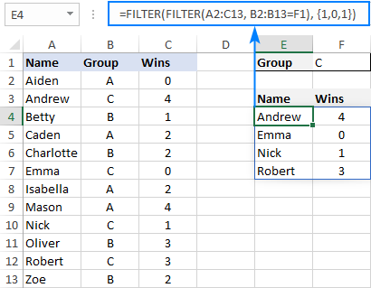
For example, to return only Names (1st column) and Wins (3rd column), we are using {1,0,1} or {TRUE,FALSE,TRUE} for the include argument of the outer FILTER function:
=FILTER(FILTER(A2:C13, B2:B13=F1), {1,0,1})
Or
=FILTER(FILTER(A2:C13, B2:B13=F1), {TRUE,FALSE,TRUE})
How to limit the number of rows returned by FILTER function
If your FILTER formula finds quite a lot of results, but your worksheet has limited space and you cannot delete the data below, then you can limit the number of rows the FILTER function returns.
Let's see how it works on an example of a simple formula that pulls players from the target group in F1:
=FILTER(A2:C13, B2:B13=F1)
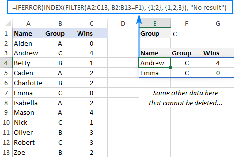
The above formula outputs all the records that it finds, 4 rows in our case. But suppose you just have space for two. To output only the first 2 found rows, this is what you need to do:
- Plug the FILTER formula into the array argument of the INDEX function.
- For the row_num argument of INDEX, use a vertical array constant like {1;2}. It determines how many rows to return (2 in our case).
- For the column_num argument, use a horizontal array constant like {1,2,3}. It specifies which columns to return (the first 3 columns in this example).
- To take care of possible errors when no data matching your criteria is found, you can wrap your formula in the IFERROR function.
The complete formula takes this form:
=IFERROR(INDEX(FILTER(A2:C13, B2:B13=F1), {1;2}, {1,2,3}), "No result")
When working with large tables, writing array constants manually may be quite cumbersome. No problem, the SEQUENCE function can generate the sequential numbers for you automatically:
=IFERROR(INDEX(FILTER(A2:C13, B2:B13=F1), SEQUENCE(2), SEQUENCE(1, COLUMNS(A2:C13))), "No result")
The first SEQUENCE generates a vertical array containing as many sequential numbers as specified in the first (and only) argument. The second SEQUENCE uses the COLUMNS function to count the number of columns in the dataset and produces an equivalent horizontal array.
Tip. To return data from specific columns, not all the columns, in the horizontal array constant that you use for the column_num argument of INDEX, include only those specific numbers. For instance, to extract data from the 1st and 3rd columns, use {1,3}.
Excel FILTER function not working
In situation when your Excel FILTER formula results in an error, most likely that will be one of the following:
#CALC! error
Occurs if the optional if_empty argument is omitted, and no results meeting the criteria are found. The reason is that currently Excel does not support empty arrays. To prevent such errors, be sure to always define the if_empty value in your formulas.
#VALUE error
Occurs when the array and include argument have incompatible dimensions.
#N/A, #VALUE, etc.
Different errors may occur if some value in the include argument is an error or cannot be converted to a Boolean value.
#NAME error
Occurs when trying to use FILTER in an older version of Excel. Please remember that it is a new function, which is only available in Office 365 and Excel 2021.
In new Excel, a #NAME error occurs if you accidentally misspell the function's name.
#SPILL error
Most often, this error occurs if one or more cells in the spill range are not completely blank. To fix it, just clear or delete non-empty cells. To investigate and resolve other cases, please see #SPILL! error in Excel: what it means and how to fix.
#REF! error
Occurs when a FILTER formula is used between different workbooks, and the source workbook is closed.
That's how to filer data in Excel dynamically. I thank you for reading and hope to see you on our blog next week!
Download practice workbook
Filter in Excel with formulas (.xlsx file)
 by
by
332 comments
Is there anyway for the "include" part of the formula to be based on multiple criteria in the same column? Using the first example in your article, could I make the filter array return all of the "b" and "c" into one output?
Hello!
Pay attention to the following paragraph of the article above: Filter with multiple AND criteria.
Hope this is what you need.
Oaky - sorry - I read that again carefully. I had missed the "Or Logic" section initially. Thanks so much - that scenario fits perfectly!
Hi!
Is it possible to use this formula to filter multiple sheets? Do i need to apply it together with VBA loop through multiple sheets?
Thanks.
Hello!
The FILTER function works only with one data area. Perhaps this article will be useful for you: Consolidate in Excel: Merge multiple sheets into one.
I'm trying to filter the data but be able to edit the data that's filtered. With dynamic filtering it's a preview of the data in the table. How do I edit the data that's filtered with dynamic filter?
Hi!
You need to edit the data in the cells in which they are written.
Hi, Thank you for such wonderful explanations with examples.
I have a question related to limiting the number of rows returned by FILTER.
In my code I have used something like this to return data consisting of limited columns (columns 1 and 3 in code with {1\3}) but with unlimited rows.
How and where should my condition for limiting the number of rows go in the following code
=FILTER(INDEX(mD!D9:F19;SEQUENCE(ROWS(mD!D9:F19));{1\3});(mD!X9:X19=TRUE)).
I tried adding the rows before the {1\3}, but it did not work.
Since the code I have has construction FILTER(INDEX...) different from the example here INDEX(FILTER...), I am not able to interpret the solution
Thank you for the update and this wonderful article. If I could ask a question:
Is it possible to loop through a column of values for the criteria? For example, if I have something like this:
Sheet2.Range("A2").Formula2 = "=FILTER(Sheet1!A2:J100,Sheet1!B1:B100=F1,"")"
Is there anyway of looping through the values in the Column F directly or say in a VB macro?
A VB macro might look like this:
Sub Test()
With ActiveSheet
Sheet2.Range("A2").Formula2 = "=FILTER(Sheet1!A2:J100,Sheet1!B1:B100=F1,"")"
End With
End Sub
The data I'm filtering can have multiple lines within a single cell. How can I set the workbook to autoFit the height when the data is pulled in?
Can you please help me to "Filter on blanks". The data set has
Column A has a list of Names
Column B has performance grades 1-5 (of which some will be blank, so if column B is blank return the corresponding Name.
=FILTER('Line by Line Data'!$A:$A,'Line by Line Data'!B:B="","") currently returns the following. What I am after is the data without 0
0
Bob Smith
0
0
0
0
Jane Evans
Hello!
If you want 0 not to be shown in empty cells, use the custom number format
###
I hope I answered your question. If something is still unclear, please feel free to ask.
Can you please help me to "Filter cells containing specific text" from multiple worksheets or multiple tables?
For example, FILTER(array, ISNUMBER(SEARCH("text", range)), "No results"). How can I added multiple tables that are in various worksheets to the above formula?
Hope someone helps. Thank you
Hello!
The FILTER function works only with the data of the current sheet. You can combine data from multiple sheets into a current sheet using the Copy Sheets tool.
It is available as a part of our Ultimate Suite for Excel that you can install in a trial mode and check how it works for free.
To work with multiple tables on one sheet might be helpful - "Example 1. Filter multiple columns in ExcelExample 1. Filter multiple columns in Excel". Read if above.
Hi Alexander - thanks for the article, I've found the FILTER function very useful for parsing data.
I'm trying to apply your does not equal logic to exclude rows of data that contain specific names. For example: =FILTER(A1:H2500,(H1:H2500(("Acme Inc."))))
This works well for a single instance like "Acme Inc.", but I would like to nest this so that I can exclude several companies tagged within column H (eg "Acme Inc."; "Smith Inc."; "Alex Inc.";). Is there a way to do this? I've tried creating an OR statement with the names with no success.
Any help is much appreciated.
To clarify, the function above should read =FILTER(H1:H2500,(H1:H2500(("Acme Inc.")))) ...regardless I have not found a way to nest multiple names from the same column.
Hello!
If I understand your task correctly, the following formula should work for you:
=FILTER(A1:B30,(A1:A30<>"Acme Inc.")*(A1:A30<>"Smith Inc.")*(A1:A30<>"Alex Inc."))
Hope this is what you need.
Hello.
I have a question.
Is possible to use filter to return image/icon?
I have a icon with a link attached in each row of my table and when I filter the table I would like that the icon also to appear in the result table...
Is it possible with FILTER?
Thank you.
Hello!
The filter works with data that is written in a cell. The icon is attached to the cell. Therefore, the filter does not see it.
Not a question, but i just wanted to say that
1) This is excellent (particularly when you match with [0,0,1,1,0,1...} to return specific columns, and
2) Wrapping FILTER in a SORT function is particularly useful in my context.
I can see all sorts of possibilities forreturning dynamic tables based on user-chosen check boxes (for example).
Now i just need to work out how to identify unique strings of text within other strings of text in filtered array! But ill get there
Hello!
Please have a look at this article — Excel unique values: how to find, filter, select and highlight
I hope it’ll be helpful.
Thanks Alexander, i have looked here and cant quite work out exactly the right formula to give me the asnwer i need. I have left a question on that thread though.
The most basic example of my problem is, i have 2 cells, lets say "1, 2" and "1, 3". I need to count the unique strings within those cells so im counting 1, 2, and 3 a single time each.
Hi,
This formula is amazing!! I have one problem though, my original data is in a separate workbook. When I first added the formula (to my new workbook) it filtered perfectly, but over time the original data changes, more rows gets added all the time, but the filter formula doesn't update to include those new rows, even when they meet all the criteria. I have set the array (in the formula) to be really big, to allow space for the new rows. Is this because its in a different workbook? Or could it be how I have saved it? Or is it because once it has been saved it doesnt update anymore?
Thank you
Rene
Hello!
In order to update the data, all the necessary files must be opened in Excel. Or click the "Refresh All" button in the Data menu
Hi,
Hope you are all well.
I am a bit stuck. I am using INDEX and FILTER to list job numbers per site. My problem is that some sites have more job numbers raised against them than others, so to try and not have the spreadsheet huge and then having to scroll down loads, id like to have 2 columns for the job numbers.
One site may have 14 job numbers, and I have limited it to show only 10, but I would like the remaining 4 to then overflow onto the column next to it, so all job numbers are still visible
Is this possible?
Many thanks in advance
Hello!
I kindly ask you to have a closer look at the following paragraph of the article above - How to limit the number of rows returned by FILTER function. It contains answers to your question.
If something is still unclear, please feel free to ask.
Hi Alexander,
I had already read that, I have limited how many jobs numbers it shows, but I am in need of the remainder be shown in the column next to it.
Example:
I have 20 cells, over 2 columns, I have 14 job numbers, 10 of the job numbers are shown in the 1st column, the remaining 4 I want to show in the 2nd column. So where all the job numbers don't fit in the 1st column, they overflow into the 2nd column.
Many thanks in advance
Hello!
You can specify numbers from 10 to 20, etc. in the formula. For example:
=IFERROR(INDEX(FILTER(A2:C13, B2:B13=F1), {10;11;12;13;14;15;16;17;18;19}, {1,2}), "No result")
Thanks for the wonderful guide ,
However , I had a doubt. Is there any method that can provide me all the outputs (matches) in one blank cell instead of a list ?
To put things into context , I have data in rows A2 to G12345 , I am looking for multiple matches against a Customer ID (having multiple occurrences) . I would therefore not want another list being shown as the output , instead , want to have all matches in cell J2 and if possible , separated by commas ? . Maybe a combination of formulas could do the trick ?
Hello!
To combine FILTER results in one cell, use the function TEXTJOIN.
For example:
=TEXTJOIN(",",TRUE,FILTER(A2:A13, B2:B13=F1, ""))
Hope this is what you need.
Hi, greetings and thanks for those good examples on FILTER.
Hope to clarify, when I selected any cell within the range of E4:G7 in worksheet "Basic FILTER formula", I noted that the whole range gets a "border" around it. And I think this is not a named range. May I seek for advice what's that about and how to do that? I noted when I selected the whole range of E4:G7, the name box showed E4#. What did that mean and the function of it?
Appreciate for you guidance and thanks again.
Hi James,
A range highlighted with a blue border is called a spill range. It is created by Excel automatically when you use a dynamic array formula that returns multiple values like our FILTER formula. A spill range indicates that everything inside it is calculated by the formula in the topmost cell.
E4# is a spill range reference that refers to the whole spill range. Unlike a regular range reference, a spill range ref is dynamic and automatically reflects changes in the range size.
All this is part of Dynamic Arrays functionality introduced in Excel 365.
For more information, please see Excel spill range explained.
Thanks so much for the update. I shall read through more on the spill range and revert if I need further guidance.
Hi @Svetlana, thanks so much. I read through the guide and it is now working and I clearly understood how it works.
Hi,
Any way to filter out specific columns without using the {1,0,0,0,1,…………} format? Would be helpful if one could use a match on column name instead somehow.
Thanks!
If source data is in a table named tbData to do this I use xmatch( "range of list of columns to match", tbData[#Headers] ). You can then pick which columns to include and they can be in a different order to the columns in the original table. Hope this helps.
How to Excel 365 Filter with indirect array of addresses not continuous:
=FILTER(INDIRECT({"$M$2";"$N$2";"$O$2";"$P$2";"$Q$2";"$R$2"}),
INDIRECT({"$M$2";"$N$2";"$O$2";"$P$2";"$Q$2";"$R$2"})""
)
Intermediate Formula Evaluation shows:
=
FILTER(
{"test5";#VALUE!;"test6";"";0;0},
{"test5";#VALUE!;"test6";"";0;0}""
)
Final output shows #VALUE! instead of non-blank cell values.
Thanks Ahead!
I'm going crazy trying to figure out why I don't have access to the FILTER() function in Excel. I have MSFT 360 and have tried using both the "Beta Channel" and "Current Channel (Preview)" and neither update has installed the FILTER() function. I found an old article that referenced Microsoft 360 "Pro" but don't see any place to purchase that on the Microsoft website, just "family" or "business" editions. AFAICT, there's no difference in functionality on those versions, only the number of people who can use it. Can you please let me know what version I need in order to access this function or, perhaps, a workaround with a different function?
Thank you!
BTW, my Excel version is 16.50 if that helps
Hi,
If you really have an OFFICE 365 subscription, then the filter function should be there. You can read about this in more detail here.
Thanks for your super fast reply. Yeah . . . it's a head scratcher for sure . . . I definitely have a 360 subscription (can log in and verify). Maybe it's because I'm running it on a Mac. Oh well. :(
Hi,
Unfortunately, I cannot help you here. But the FILTER function is also available on Mac. Look carefully at the link I gave you. FILTER is currently available to Microsoft 365 subscribers in Current Channel.
Hi, Excellent info on the filter function... saved me many weeks of work!
I wonder if you could help me on this:
Am applying a filter on a price list, to return a set of products based on the type of category - and this works fine. But now I would like to eliminate rows which have become "obsolete" since price has changed. For example I have this data set:
PRODUCT - PRICE - LAST PRICE CHANGE
Coffee Brand A - $5 - 1/1/2020
Tea Brand X - $1 - 5/12/2020
Coffee Brand B - $4 - 1/5/2021
Coffee Brand A - $6 - 4/30/2021
I would like my output to IGNORE the first row, dated 1/1/2020 since the price for that brand (Coffee Brand A) has now changed on 4/30/2021.
Is there a way to achieve this dynamically? I would need to include this as part of the FILTER function, since the table above would have been "built" by using a filter on the category called "Tea&Coffee".
Thank you!
Hello!
Please try the following formula:
=FILTER(A1:C6,(D1:D6="category")*(C1:C6=MAXIFS(C1:C6,A1:A6,A1:A6)))
You can learn more about MAXIFS function in Excel in this article on our blog.
Hi,
I tried the formula and it worked perfect in selecting the correct row from the two dates. The problem I have is that I want all records to be returned, except the "obsolete" one. To use my example again:
The full list is this:
PRODUCT - PRICE - LAST PRICE CHANGE
Coffee Brand A - $5 - 1/1/2020
Tea Brand X - $1 - 5/12/2020
Coffee Brand B - $4 - 1/5/2021
Coffee Brand A - $6 - 4/30/2021
Your suggested equation returned:
PRODUCT - PRICE - LAST PRICE CHANGE
Coffee Brand A - $6 - 4/30/2021
What I would like to return is this:
PRODUCT - PRICE - LAST PRICE CHANGE
Tea Brand X - $1 - 5/12/2020
Coffee Brand B - $4 - 1/5/2021
Coffee Brand A - $6 - 4/30/2021
Can you suggest a modification please?
Thank you so much for your help.
I think I found a workaround: I introduced a column which flags whether that row is "obsolete" or not. Then used an "*" in the filter to check against it.
Equation now looks like this:
=UNIQUE(FILTER(FILTER(T_PRI, (Table2[[#All],[CATEGORY]]=B17)*(Table2[[#All],[OBSOLETE]]="")),{1,1,1,1,0,1,1,0,0,0,1,1}))
Hello!
The formula I sent to you was created based on the description you provided in your first request.
You wrote: "Am applying a filter on a price list, to return a set of products based on the type of category". If you need a complete list, then remove this condition from the filter.
=FILTER(A1:C10,(C1:C10=MAXIFS(C1:C10,A1:A10,A1:A10)))
Hope this is what you need.
Hello
Great tutorial.
one more question: How to filter with the new FILTER-function multiple criteria (AND, OR) with wildcard(s), in a table column
e.g.
Table:
Col A Col B Criteria for search in Language column: Result:
Row 1 Country Language ma (eg. in cell D1) Germany german
Row 2 Germany german re (eg. in cell D2) France french
Row 3 France french isc (eg. in cell D3) Spain spanish
Row 4 Italy italian
Row 5 Spain spanish
Hello!
If I understand your task correctly, pay attention to the following paragraph of the article above — Filter cells containing specific text
Hope this is what you need.
Thank you very much for your reply. That is correct, however I am locking for a possibility to enter more than one search string as in my example above mentioned (the format of the example was lost when transmitting the post that is why it is not easy to read)
- The Table is in Col A and B Row 1 to 5 named Countries
- The headers of the table are named "Country" and "Language"
- The Search Strings (only part of the words in the table) are in Column D Row 1 to 3 (ma, re, isc - who are in normal search with wildcards "*" or "?")
- The Filter-Function for the result should be in Cell "F1” (the search should be an “OR” search how would it be with an “AND” search ?
How to distinguish in the Filter Function between exact match, with Wildcard “*” or with Wildcard “?”
Hello,
FILER function for more than one criteria:
After long trials I got now the answer for filtering more than 1 Criteria in a PowerQuery Table.
1. I have to define a named range for the search area, then define the FILTER formula
2. Execute the PowerQuery and put it to the in the FILTER formula defined range.
With this I am able to run the FILTER function with more than 1 criteria
Eg.
For Criteria 1 AND 2
=FILTER(A2:H656;(ISTZAHL(SUCHEN(L2:L2;Betreff))*ISTZAHL(SUCHEN(L3:L3;Betreff)));"kein Resultat")
For criteria 1 OR 2
=FILTER(A2:H656;(ISTZAHL(SUCHEN(L2:L2;Betreff))+ISTZAHL(SUCHEN(L3:L3;Betreff)));"kein Resultat")
For criteria 1 AND (2 OR 3)
=FILTER(A2:H656;(ISTZAHL(SUCHEN(L2:L2;Betreff))*ISTZAHL(SUCHEN(L3:L3;Betreff))+ISTZAHL(SUCHEN(L4:L4;Betreff)));"kein Resultat")
Ps.
ISTZAHL equals Isnumber
SUCHEN equals SEARCH
Betreff is the named search range
For changing between the 3 Filter options (FILTER function) I wrote a macro which changes the FILTER formula automatically
Hello!
Sorry, it's not quite clear what you are trying to achieve.
The SEARCH function does not use wildcards. Which formula do you want to use?
Please specify what you were trying to find, what formula you used and what problem or error occurred. Give an example of the expected result.
It’ll help me understand it better and find a solution for you.
1. how to filter based on checkbox that contain cell value from table in different sheet?
2. how to filter based on drop-down that have VBA code which helps to click multi selections that contain cells value from table in different sheet?
Is there a way to use =FILTER across multiple worksheets in a single formula? I'm using it to pull rows that meet certain criteria, but the reports I have to work with can have many worksheets to sift through.
An example:
=FILTER(Sheet1!A6:J1667,(Sheet1!G6:G1667="VariableX")+(Sheet1!G6:G1667="VariableY")+(Sheet1!G6:G1667="VariableZ"),"")
Currently I am pasting a new =FILTER formula below the lowest returned line:
=FILTER(Sheet2!A6:J1667,(Sheet1!G6:G1667="VariableX")+(Sheet2!G6:G1667="VariableY")+(Sheet2!G6:G1667="VariableZ"),"")
And so on for how ever many sheets there happen to be. If I was able to build in [filter Sheet1 then also filter SheetN+1 until they are all filtered], it would save me a good deal of time.
Hi Alexander!
I am mixing up rows and columns some how but found that Svetlana had replied in an earlier question that I could use to get what I was looking for. Only returning specific columns.
FILTER(FILTER(A2:C13, B2:B13=F1), J1:L1) :)
It did!! Thank you Alexander!
Could you see why this works and filters.
FILTER(Data!A:G;Data!G:G="Covid";"No results")
While this doesn't.
FILTER(FILTER(Data!A:G;Data!G:G="Covid";"No results");{1;0;0;1;1})
I constantly get #VALUE!
Jen
Hello!
The criteria in the FILTER function must return TRUE or FALSE. Your values {1;0;0;1;1} don't.
Pay attention to the following paragraph of the article above - Filter with multiple AND criteria.
I hope it’ll be helpful.
Great tutorial!
One thing I don't see solved is as for my case.
I have cell values that sometimes have data and sometimes they are empty.
I am using the cells for input to my Filter function.
A B C D
1 Month Article Cost Owner
2 202103 John
FILTER(array, (range1=criteria1) * (range2=criteria2), "No results")
FILTER(array, (range1=202103) * (range2=)* (range3=)* (range4=John), "No results")
In the case I don't have any input criteria as in Column B and Column C above.
It will send the input filter-out-all-rows-where range 1= 202103, range 2=empty, range 3=empty, range 4=John
How do I get around that I want to have the possibility to use all criterias but sometimes they are empty.
I currently have 11 cells that I would like to use for criterias.
Thank you!
Hello!
Add additional conditions to check an empty criterion cell.
FILTER(array, ((range1=criteria1)+(criteria1="")) * ((range2=criteria2) + (criteria2="")), “No results”)
I hope my advice will help you solve your task.
I am using a Filter list to populate another sheet. Based on the names that appear in this new list, I am writing some static formulas/remarks. The problem I am having is that when the Filter list updates, sometimes the new data/names appear ON TOP of the original list, due to which the static data no longer matches with that which was imported from the Filter List. Is there any way to add the new entries from the filter list at the bottom? Or to tie the static data to the dynamic data?
I have an excel column that contains text in around 1000 cells. In each cell, some text is BOLD, some text is ITALALICS, and some text is in REGULAR fonts. Thus, each cell has all three fonts (bold, italics & regular) in it.
I want to filter cells that contain the text "because" in bold fonts only.
Can you please help to write FILTER FORMULA for this.
Yours sincerely,
Prakash Dave.
Hello!
Your formatting does not change the "TEXT" format of the cell. Therefore, using Excel formulas, your task cannot be completed.
Is there any way of using array as criteria in a Filter function?
For instance, in your SUM, AVERAGE... examples - instead of F1 providing the Group as the criteria, calculate SUM for {"A","B","C"...}. The array could have been created using UNIQUE. And so the the output of the SUM will be an array.
I have a similar problem, and I'm just getting error messages.
Hello!
For me to be able to help you better, please describe your task in more detail. Please specify what you were trying to find, what formula you used and what problem or error occurred. Give an example of the source data and the expected result.
It’ll help me understand it better and find a solution for you.
Hi,
I'm referring to the section in this webpage titled: "Filter and calculate (Sum, Average, Min, Max, etc.)"
I want to have something like the following formula:
=SUM(FILTER(C2:C13,B2:B13=UNIQUE(B2:B13),0))
Source data is as per the section in the webpage.
My aim is to get results that show:
Group, Wins
A, 8
B, 11
C, 5
...and for it to be generated dynamically without knowing beforehand how many groups there are in the source data.
I get #N/A when I try this.
Hello!
The FILTER function cannot compare two arrays. You can use these formulas:
In cell E4:
=IF(SORT(UNIQUE(B2:B100),1,1)=0,"",SORT(UNIQUE(B2:B100),1,1))
In cell F4:
=IF(E4<>"",SUM(FILTER(C2:C100,B2:B1100=E4, 0)),"")
Copy this formula down along the column F.
I hope my advice will help you solve your task.
Thanks for that, Alexander. It is useful to know what FILTER *can't* do.
Is there anywhere that clearly documents the *details* of the new(ish) array and dynamic array functionality? It seems to be a lot for trial and error and searching various blogs.
I'm looking for something that better explains the interfaces - i.e. where you can and can't use them.
By the way, there's a slight typo in your formula for cell F4 it should read:
=IF(E4"",SUM(FILTER(C2:C100,B2:B100=E4, 0)),"")
Hello
I was wondering if there is any way to automatically insert rows if the filtered data requires more space than available. I was thinking about a dynamic page break which increase and decrease with the data required to be displayed.
Please advise.
Thanks
Z
Hello,
I am not sure if the "filter" function is the most appropriate, I think I would have to use a combination of functions for my case. So, my dataset looks like the one below.
Zone 1 2 3
a 13 12 75
b 98 0 2
c 0 100 0
I need to remove the "0" values and for zone 1 create as many rows as values I have. So, the final format should look like the following,
Zone
1 13 a
1 98 b
2 12 a
2 100 c
3 75 a
3 2 b
Could you please suggest me how to do that?
Can the input range to a listbox form control be the spill range of =UNIQUE(....)?
I want the input range to a list box form control to be all the DIFFERENTsales reps in column A without duplicates.
Hello!
Extract unique data to any empty column. Use this instruction.
Then, using the formula, get a list without empty cells:
=OFFSET($D$1,,,COUNTA($D$1:$D$200))
Copy the entire formula from the formula bar.
Select cell, which is where you want the dropdown to be shown.
Go to Data > Data Validation.
Paste the formula as the Source.
I hope I answered your question. If something is still unclear, please feel free to ask.
I'm trying to use a range from another sheet for the array and criteria. It looks like this:
=UNIQUE(FILTER('Sheet1'!A2:B220,('Sheet1'!E2:E219 "")))
I'm getting a #Value error. Does referencing other sheets just not work?
Hello!
Unfortunately, without seeing your data it is difficult to give you any advice. But the FILTER function was used with an error. Please check out the following article on our blog, it’ll be sure to help you with your task: Get a list of unique values based on criteria.
I hope I answered your question. If something is still unclear, please feel free to ask.
I actually figured out the problem and have it working now. But I have a new question. Is there a way to just have it check every sheet in the workbook? Here is my formula now (each sheet is a date):
=UNIQUE(FILTER('14-01-21'!A2:B219,('14-01-21'!E2:E219"") + ('18-01-21'!E2:E219"") + ('20-01-21'!E2:E219"") + ('21-01-21'!E2:E219"") + ('25-01-21'!E2:E219"") + ('27-01-21'!E2:E219"") + ('28-01-21'!E2:E219"") + ('01-02-21'!E2:E219"") + ('02-02-21'!E2:E219"") + ('04-02-21'!E2:E219"") + ('08-02-21'!E2:E219"") + ('11-02-21'!E2:E219"")))
As you can see, this is really messy. The other problem is, new sheets will be added as time goes on. That's why I'm wondering if there's a way to have it check E2:E219 in every sheet rather than having add each sheet individually.
Thank you for this great article. I just wanted to ask if it is possible to filter using multiple columns in the expression, i.e. =FILTER(A2:C10,ISNUMBER(SEARCH(F2,B2:C10)),"No Results").
You see I have 3 columns and I want to display all rows that contain the Keyword in either Columns B or C.
Thanks.
Hello!
Pay attention to the following paragraph of the article above - Example 1. Filter multiple columns in Excel
=FILTER(A2:C13, (B2:B13=F2) * (C2:C13=F2), "No results")
I hope it’ll be helpful.
Hi thanks for detailed explanations and enormous work you guys put to create this resource! I have a quick question:
For instance I have a list of t-shirts. I want to filter t-shirts by color and price ("blue" and "above 5 dollars"). However, I at the same filter I want also give my users an option to filter ALL colors of t-shirts above 5 dollars. What could be the solution? I tried to use IF statements or AND/OR in my formula, but I could not succeed maybe I am doing something wrong. Thanks for your answers!
Hello!
I hope you have studied the recommendations in the tutorial above. It contains answers to your question.
=FILTER(A2:C7,B2:B7="blue")
=FILTER(A2:C7,(B2:B7="blue")*(C2:C7>5))
=FILTER(A2:C7,C2:C7>5)
A- name, B - color, C - price
Thanks for your answer Alexander! Unfortunately, your solution requires 3 separate formulas. However, I want to give an option to filter "all colors" as well as individual colors in the same formula.
=FILTER(A2:C7,(B2:B7="{blue, red, yellow, all colors}")*(C2:C7>5)).
I want to give a user something like drop down list where he/she can select color from the list "blue", "red", "yellow" as well as "all colors". I can do individuals colors, but I can not do "all colors" option. I also tried to use "*" symbol, but FILTER function does not support wildcards.
I would appreciate your comment/solution to this problem! Thanks!
Hi,
To select all colors or multiple colors in the filter, study this paragraph above — Filter with multiple criteria
Hi Alexander,
Thanks for your comments and help to master excel. I was able to figure this problem out using IF statements together with FILTER function. Just in case anybody came across with a similar situation below how I solved the problem:
Step 1.: I created a table with color and prices for T-shirts (i.e. I3"BLUE", J3"12"; I4"RED",J4 "10"; I5"GREEN", J5"5" AND I6"ALL COLORS", J6"0")
Step 2.: I created a two data input table 1 for Price (B1) and one for Color where you can select individual colors and "ALL COLORS" from the drop down list (I used Data Validation- List).
Step 3. I created a below formula in cell A4:
=IF(B2"ALL COLORS",FILTER(I3:J6,(J3:J6>B1)*(I3:I6=B2)),FILTER(I3:J6,(J3:J6>B1)))
Basically the logic of formula goes as the following:
If color is not selected as "ALL COLORS", then filter table based on Price and Color, else filter based on Price only.
Now I can filter T-shirts based on individual colors as well as price only. I know it might sound simple but it took me few days to research and think about it.
I would be happy if this could help to save someone's time! Have a great day! :)
Hi,
excellent article, thank you.
I have multiple data points for several individuals re-occuring on different dates. I am able to filter out the specific people I want based on certain criteria, but can I also get an average of their score for each day.
Thanks,
Paul
Hi, I love all the examples! Do you know if FILTER can be used directly in data validation source?
That is, I would like to have a drop down list with items depending on selection in another dropdown list.
I tried this formula in cell AB3:
=FILTER(B1list;$AA$3=BtoB1;"")
and it works nicely in a cell, but when I try to use it in data validation --> list --> source it says 'The Source currently evaluates to an error".
(AA3 is where the user is supposed to select the first value and I would like them to only see relevant items from the list BtoB1 list in cell AB3)
Cheers,
Kamil
Hi Kamil,
We have a special article on this - Create a dynamic dependent dropdown list an easy way. Hope you will find it helpful.
Hello!
Unfortunately, without seeing your data it is difficult to give you any advice. Please check out this article to learn how to create a cascading drop down list
Hello, excellent article, thanks!
Is there any way to limit the number of rows a FILTER function returns? For exmaple, the function returns 10 rows but I have only space for 5 (and I cannot delete the data below that)... is this feasible?
Thanks!
Hello!
What an interesting question! Yes, it is possible, and I have created a separate example for other users to know :)
Please see How to limit FILTER results
Hi,
Probably an easy question:
If we look at the example: Basic Excel FILTER formula.
I would like to have A AND B if F1 is empty, is that possible?
Thanks in advance.
Great post! This is so powerful and I learned so much!!
Is there a way to Filter Non-Adjacent Columns and define the Array Constant using a formula (or in some way dynamically)?
Here's what I mean: I would like the {1,0,1} to change to {1,1,0} based on other criteria in my workbook.
=FILTER(FILTER(A2:C13, B2:B13=F1), {1,0,1})
Can change to:
=FILTER(FILTER(A2:C13, B2:B13=F1), {1,1,0})
Is this possible?
Thanks again for this great post!!!!
Hi!
It' difficult to say anything certain without knowing exactly what kind of criteria you have in your workbook. Anyway, I believe the simplest approach that you can try is nested IFs.
For example, if K1=1, return {1,0,1}, if K1=2, then return {1,1,0}:
=IF(K1=1, FILTER(FILTER(A2:C13, B2:B13=F1), {1,0,1}), IF(K1=2, FILTER(FILTER(A2:C13,B2:B13=F1), {1,1,0}),""))
Thank you Svetlana. That is not quite what I'm hoping to accomplish. I would like to create the Array Constant Dynamically. So in this example, cells A1, A2, A3 might contain 1's and 0's that would be used to populate the Array Constant. So if A1=1, A2=0, and A3=1, the Array Constant would be {1,0,1}
In short, I would like to build the {1,0,1} parameter using a formula.
Is this possible?
Thank you again! SJ
Oh, that makes things even easier :)
Instead of an array constant, you can use a regular range reference. For example:
=FILTER(FILTER(A2:C13, B2:B13=F1), J1:L1)
Where J1:L1 are the cells containing your 1 and 0 values.
OMG Svetlana you are the absolute best!!!!
One more question. This works when I use a horizontal range but not when I use a vertical range. Just curious why? And any way I can work around this?
As an example:
=FILTER(FILTER(A2:C13, B2:B13=F1), J1:L1)
works fine
=FILTER(FILTER(A2:C13, B2:B13=F1), J1:J3)
does not
Thank you so much - this has save me countless hours!!! You are like an Excel Angel!!!
Thank you :)
As for your question, it's because {1,0,1} is a horizonal array, so it requires a compatible horizontal range.
If your data was organized horizontally in rows (i.e. if you transposed your table), then the FILTER formula would require a vertical array constant like {1;0;1} to return data from specific rows. And you would replace that array constant with a vertical range.
We have a couple of in-depth tutorials on Excel arrays and traditional CSE array formulas. If you are curious, you can check them out:
Excel array formulas, functions and constants (among other things, it explains the difference between vertical and horizonal arrays)
Excel array formula examples for beginners and advanced users
So how do you make it work with VBA.
With the first example I used =FILTER(A2:C13,B2:B13=F1,"No Results") in excel and it worked as shown.
Next I created a macro and it FAILED!!!!
Here is the macro
Sub test()
Range("I4") = Filter(Range("A2:C13"), Range("B2:B13") = F1, "No Results")
End Sub
Run-time error '13': Type mismatch
Hello, your guides are amazing.
I have a question: is it possible to connect two filter arrays es.
FILTER #1:
a - 1
b - 2
c - 3
FILTER #2:
d - 4
e - 5
Connected Filters:
a - 1
b - 2
c - 3
d - 4
e - 5
Thank you :)
I mean without VBA
Hello!
If I understand your task correctly, pay attention to the following paragraph of the article above — Filter with multiple criteria (AND logic)
If this is not what you wanted, then please clarify your question in more detail.
Thank you for the answer.
I mean another thing:
I have 2 different starting matrix that I filter with the FILTER function.
In the way I obtain 2 different filtered matrix.
FILTERED MATRIX #1
a - 1
b - 2
c - 3
FILTERED MATRIX #2:
d - 4
e - 5
What I would like to obtain is a new (dynamic) matrix that is the fusion of the two filtered matrix.
ES. OF THE FINAL MATRIX:
a - 1
b - 2
c - 3
d - 4
e - 5
Without using VBA
Hello!
If I understand your problem correctly, you want to combine the results of the two filters. You can use the recommendations from the section above — Filter with multiple criteria (OR logic)
Hope this is what you need.
Not exactly.
As I said the starting matrices are two and are different, so the FILTER functions refers to different matrices.
Here is an exemple:
=FILTER(A1:B10;A1:A10=5)
=FILTER(AA1:BB10;AA1:AA10=5)
As you can see the starting matrices are different (A1:B10 and AA1:BB10)
What I want is to combine the resulting arrays into a single matrix.
In other words how can I "merge" two different matrices into one, without using VBA?
Hello!
Merge an Excel spreadsheet using formulas is not possible in your case. You can learn more about it in this article.
We have a ready-made solution for your task - Copy Sheets Wizard. It is available as a part of our Ultimate Suite for Excel that you can install in a trial mode and check how it works for free.
If there is anything else I can help you with, please let me know.
Thank you Alexander
I believe you were looking for something like this:
={FILTER(Sheet1!F2,Sheet1!F2:F0);FILTER(Sheet2!F2,Sheet2!F2:F0);FILTER(Sheet3!F2,Sheet3!F2:F0)}
This will return a filtered list of all 3 sheets.
Works like a charm in Sheets, I'm still trying to figure out how to make it work in excel.
Is it possible to use the Filter Function to filter on format, in this specific case, color? I'm trying to avoid VBA for this specific workbook.
Thanks
Hello!
Please have a look at this article: How to filter cells by color in Excel
See also this article.
Hope you’ll find this information helpful.
I'm trying to enter this function into an xlsm sheet whic has other macros. However, it is returning error #Value... any help would be really appreciated
Im unable to upload my file or could have shared the same as well
Hello!
Check the data in the cells you are referencing. Do they match the value in the filter?
Please specify, what formula you used. Give an example of the source data.
It’ll help me understand your request better and find a solution for you.
See also this section above.
Dear Sir,how to filter data ,(Like Company Record of Daily Expanse to Employees,i want to select only one date and the all associated data of that day will show by choosing date)
Hello!
If the required date is written in a cell (for example, F1), then you can use the formulas from the second section of this article. If you want to write a date into a formula, use the DATE function.
I hope I answered your question.
Regarding using aggregate functions wrapped around filter results ... set {is empty] to zero works fine for most aggregate functions such as SUM, but is problematic for COUNT functions. The intention behind wrapping the filter function with COUNT is to count rows. If no rows exist matching the filter criteria, then , I want the COUNT function to return zero. Maybe I am missing something, but this is a lot harder to do than I thought. Maybe I need to abandon the FILTER and UNIQUE function to use other methods. Any suggestions? Thanks
Hello!
You have not listed the formulas that are causing the problem. But I think using function IFERROR will help replace the error message with zero.
If there is anything else I can help you with, please let me know.
How do i create a filter on an ever changing range (sometimes 100 rows, sometimes 250, or even 10) - do i have to preset the filter to cover x number of rows, or can i create dynamic range
Hello!
If you are using the FILTER function, then I recommend using a dynamic named range or Excel table.
Hi Alexander,
Can we filter by connecting to a dynamic range via a pivot table?
Hello!
Please have a look at this article — Excel slicer: visual filter for pivot tables.
I hope my advice will help you solve your task.
With is formula I pull all rows for the week and corresponding times. I sort on the week. Is it possible to add a blank line to separate each day of the week? My spreadsheet has 85 columns, I show column 1 (date) and column 2 (key time). I also need sort both the Date and Key Time. Thank you for any assistance.
=FILTER(SORT(FILTER(TDaily[[Date]:[Key Time]], (TDaily[Date]>=I10) * (TDaily[Date]<=I11)), 1, 1), {1,0,0,0,0,0,0,0,0,0,0,0,0,0,0,0,0,0,0,0,0,0,0,0,0,0,0,0,0,0,0,0,0,0,0,0,0,0,0,0,0,0,0,0,0,0,0,0,0,0,0,0,0,0,0,0,0,0,0,0,0,0,0,0,0,0,0,0,0,0,0,0,0,0,0,0,0,0,0,0,0,0,82})
Hello!
The FILTER function returns an array of values. Therefore, it cannot return any empty lines. If you create a pivot table from this data, then different formatting methods are possible there.
Hi Lady,
Is it posible to filter if a column matches any of a list of values.
Example:
List of criterias
A1: 1
A2: 2
A3: 3
A4: 4
The data i want to filter:
B1: 1
B2: 4
B3: 3
B4: 6
B5: 7
B6: 2
=FILTER(dataToFilter, dataToFilter=listOfCriteria, "No results")
Result:
1
4
3
2
is there a way to do this?
Thanks in advance!
Hello!
I kindly ask you to have a closer look at the following paragraph of the article above Filter with multiple OR criteria
Hello 👋 , i install office 2021 but filter function is not available in the functions, can you help me? Please
Hi,
In your examples, how do you return just Name and Wins for example
Hi Matt,
This is an excellent question. Thank you for asking! I've added this example to the tutorial, please see How to FILTER non-adjacent columns.
Hello!
One doubt:
How do I Add a last row with column sum, using filter? Could I do that?
Hi Lincoln,
This can be done by using the SUM function with a spill range reference (# symbol).
Assuming the FILTER formula is in E4, the SUM formula will be as simple as this:
=SUM(E4#)
Just make sure there are enough empty rows between the FILTER and SUM formula cells. If FILTER does not have the required number of rows to fill with the results, a #SPILL error will occur.