The tutorial shows how to use the MAXIFS function in Excel to get the maximum value with conditions.
Traditionally, when you ever needed to find the highest value with conditions in Excel, you had to build your own MAX IF formula. While not a big deal for experienced users, that might present certain difficulties for novices because, firstly, you should remember the formula's syntax and, secondly, you need to know how to work with array formulas. Luckily, Microsoft has recently introduced a new function that lets us do conditional max an easy way!
Excel MAXIFS function
The MAXIFS function returns the largest numeric value in the specified range based on one or more criteria.
The syntax of the MAXIFS function is as follows:
Where:
- Max_range (required) - the range of cells where you want to find the maximum value.
- Criteria_range1 (required) - the first range to evaluate with criteria1.
- Criteria1 - the condition to use on the first range. It can be represented by a number, text or expression.
- Criteria_range2 / criteria2, …(optional) - additional ranges and their related criteria. Up to 126 range/criteria pairs are supported.
This MAXIFS function is available in Excel 2019, Excel 2021, and Excel for Microsoft 365 on Windows and Mac.
As an example, let's find the tallest football player in our local school. Assuming the students' heights are in cells D2:D11 (max_range) and sports are in B2:B11 (criteria_range1), use the word "football" as criteria1, and you will get this formula:
=MAXIFS(D2:D11, B2:B11, "football")
To make the formula more versatile, you can input the target sport in some cell (say, G1) and include the cell reference in the criteria1 argument:
=MAXIFS(D2:D11, B2:B11, G1)
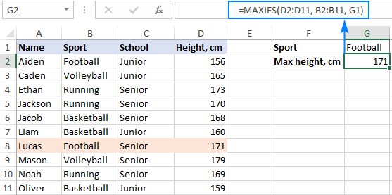
Note. The max_range and criteria_range arguments must be of the same size and shape, i.e. contain the equal number of rows and columns, otherwise the #VALUE! error is returned.
How to use MAXIFS function in Excel - formula examples
As you have just seen, the Excel MAXIFS is quite straightforward and easy to use. However, it does have a few little nuances that make a big difference. In the below examples, we will try to make the most of conditional max in Excel.
Find max value based on multiple criteria
In the first part of this tutorial, we created a MAXIFS formula in its simplest form to get the max value based on one condition. Now, we are going to take that example further and evaluate two different criteria.
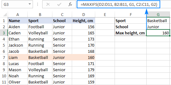
Supposing, you want to find the tallest basketball player in junior school. To have it done, define the following arguments:
- Max_range - a range of cells containing heights - D2:D11.
- Criteria_range1 - a range of cells containing sports - B2:B11.
- Criteria1 - "basketball", which is input in cell G1.
- Criteria_range2 - a range of cells defining the school type - C2:C11.
- Criteria2 - "junior", which is input in cell G2.
Putting the arguments together, we get these formulas:
With "hardcoded" criteria:
=MAXIFS(D2:D11, B2:B11, "basketball", C2:C11, "junior")
With criteria in predefined cells:
=MAXIFS(D2:D11, B2:B11, G1, C2:C11, G2)
Please notice that the MAXIFS function in Excel is case-insensitive, so you needn't worry about the letter case in your criteria.
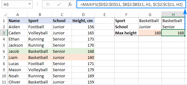
In case you plan to use your formula on multiple cells, be sure to lock all the ranges with absolute cell references, like this:
=MAXIFS($D$2:$D$11, $B$2:$B$11, G1, $C$2:$C$11, G2)
This will ensure that the formula copies to other cells correctly - the criteria references change based on the relative position of the cell where the formula is copied while the ranges remain unchanged:
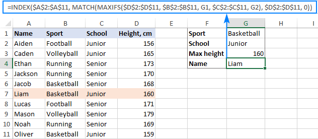
As an extra bonus, I will show you a quick way to extract a value from another cell that is associated with the max value. In our case, that will be the name of the tallest person. For this, we will be using the classic INDEX MATCH formula and nest MAXIFS in the first argument of MATCH as the lookup value:
=INDEX($A$2:$A$11, MATCH(MAXIFS($D$2:$D$11, $B$2:$B$11, G1, $C$2:$C$11, G2), $D$2:$D$11, 0))
The formula tells us that the name of the tallest basketball player in junior school is Liam:
Excel MAXIFS with logical operators
In situation when you need to evaluate numeric criteria, use logical operators such as:
- greater than (>)
- less than (<)
- greater than or equal to (>=)
- less than or equal to (<=)
- not equal to (<>)
The "equal to" operator (=) can be omitted in most cases.
Usually, choosing an operator is not a problem, the trickiest part is to build criteria with the correct syntax. Here's how:
- A logical operator followed by a number or text must be enclosed in double quotes like ">=14" or "<>running".
- In case of a cell reference or another function, use the quotes to begin a string and an ampersand to concatenate the reference and finish the string off, e.g. ">"&B1 or "<"&TODAY().
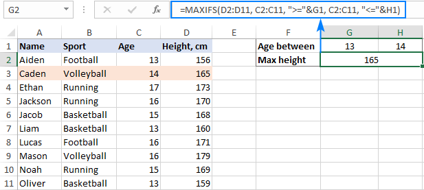
To see how it works in practice, let's add the Age column (column C) to our sample table and find the maximum height among the boys aged between 13 and 14. This can be done with the following criteria:
Criteria1: ">=13"
Criteria2: "<=14"
Because we compare the numbers in the same column, criteria_range in both cases is the same (C2:C11):
=MAXIFS(D2:D11, C2:C11, ">=13", C2:C11, "<=14")
If you do not want to hardcode the criteria in the formula, input them in separate cells (e.g. G1 and H1) and use the following syntax:
=MAXIFS(D2:D11, C2:C11, ">="&G1, C2:C11, "<="&H1)
The screenshot below shows the result:
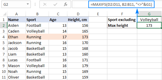
Aside from numbers, logical operators can also work with text criteria. In particular, the "not equal to" operator comes in handy when you wish to exclude something from your calculations. For example, to find the tallest student in all sports excluding volleyball, use the following formula:
=MAXIFS(D2:D11, B2:B11, "<>volleyball")
Or this one, where G1 is the excluded sport:
=MAXIFS(D2:D11, B2:B11, "<>"&G1)
MAXIFS formulas with wildcard characters (partial match)
To evaluate a condition that contains a specific text or character, include one of the following wildcard character in your criteria:
- Question mark (?) to match any single character.
- Asterisk (*) to match any sequence of characters.
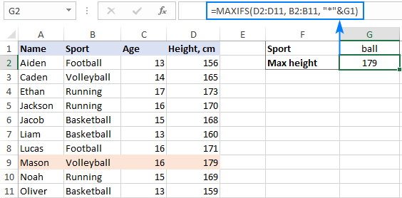
For this example, let's find out the tallest guy in game sports. Because the names of all game sports in our dataset end with the word "ball", we include this word in the criteria and use an asterisk to match any previous characters:
=MAXIFS(D2:D11, B2:B11, "*ball")
You can also type "ball" in some cell, e.g. G1, and concatenate the wildcard character with the cell reference:
=MAXIFS(D2:D11, B2:B11, "*"&G1)
The result will look as follows:
Get max value within a date range
Because dates are stored as serial numbers in the internal Excel system, you work with the dates criteria in the same manner as you work with numbers.
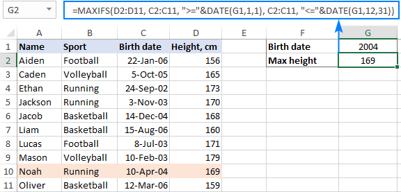
To illustrate this, we will replace the Age column with Date of Birth and try to work out the max height among the boys born in a particular year, say in 2004. To accomplish this task, we need to "filter" the birth dates that are greater than or equal to 1-Jan-2004 and less than or equal to 31-Dec-2004.
When building your criteria, it is important that you provide the dates in the format that Excel can understand:
=MAXIFS(D2:D11, C2:C11, ">=1-Jan-2004", C2:C11, "<=31-Dec-2004")
Or
=MAXIFS(D2:D11, C2:C11, ">=1/1/2004", C2:C11, "<=12/31/2004")
To prevent misinterpretation, it makes sense to utilize the DATE function:
=MAXIFS(D2:D11, C2:C11, ">="&DATE(2004,1,1), C2:C11, "<="&DATE(2004,12,31))
For this example, we will type the target year in G1, and then use the DATE function to supply the dates:
=MAXIFS(D2:D11, C2:C11, ">="&DATE(G1,1,1), C2:C11, "<="&DATE(G1,12,31))
Note. Unlike numbers, dates should be enclosed in quotation marks when used in the criteria on their own. For example:
=MAXIFS(D2:D11, C2:C11, "10/5/2005")
Find maximum value based on multiple criteria with OR logic
The Excel MAXIFS function is designed to test the conditions with the AND logic - i.e. it processes only those numbers in max_range for which all the criteria are TRUE. In some situations, however, you may need to evaluate the conditions with the OR logic - i.e. process all the numbers for which any of the specified criteria is TRUE.
To make things easier to understand, please consider the following example. Supposing you want to find the maximin height of the guys who play either basketball or football. How would you do that? Using "basketball" as criteria1 and as "football" criteria2 won't work, because Excel would assume that both criteria should evaluate to TRUE.
The solution is to make 2 separate MAXIFS formulas, one per each sport, and then use the good old MAX function to return a higher number:
=MAX(MAXIFS(C2:C11, B2:B11, "basketball"), MAXIFS(C2:C11, B2:B11, "football"))
The screenshot below shows this formula but with the criteria in predefined input cells, F1 and H1:
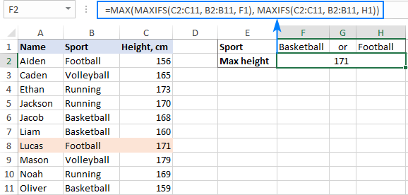
Another way is to use a MAX IF formula with OR logic.
7 things to remember about Excel MAXIFS
Below you will find a few remarks that will help to improve your formulas and avoid common errors. Some of these observations have already been discussed as tips and notes in our examples, but it might be helpful to get a short summary of what you've already learned:
- The MAXIFS function in Excel can get the highest value based on one or multiple criteria.
- By default, Excel MAXIFS works with the AND logic, i.e. returns the maximum number that meets all of the specified conditions.
- For the function to work, the max range and criteria ranges must have the same size and shape.
- The SUMIF function is case-insensitive, i.e. it does not recognize the letter case in text criteria.
- When writing a MAXIFS formula for multiple cells, remember to lock the ranges with absolute cell references for the formula to copy correctly.
- Mind the syntax of your criteria! Here are the main rules:
- When used on their own, text and dates should be enclosed in quotation marks, numbers and cell references should not.
- When a number, date or text is used with a logical operator, the whole expression must be enclosed in double quotes like ">=10"; cell references and other functions must be concatenated by using an ampersand like ">"&G1.
- MAXIFS is only available in Excel 2019 and Excel for Office 365. In earlier versions, this function is not be available.
That's how you can find the maximum value in Excel with conditions. I thank you for reading and hope to see you on our blog soon!
Download practice workbook:
Excel MAXIFS formula examples (.xlsx file)
 by
by
21 comments
In my trading journal I calculate MAXIFS and MINIFS for my trades. Often, I have a trades in a particular stock that will neither have a winner (i.e. profit) or a loser (i.e. loss). For example, if I have 4 trades in XOM, all of them could me winners. So when I calculate the largest loser using MINIFS, I get zero. Rather than getting a zero, I would like to get my answer as "N/A". How can I do this? Here's the formula I am using: =MINIFS($L$3:$L$142, $L$3:$L$142, "<0", $C$3:$C$142, $U$3, $N$3:$N$142, $U$4).
Since all my trades have been winners, I get a zero. Thank you!
Hi! To get “N/A” instead of 0, use IF function. For example:
=IF(MINIFS($L$3:$L$142,$L$3:$L$142,"<0",$C$3:$C$142,$U$3,$N$3:$N$142,$U$4)=0, "N/A", MINIFS($L$3:$L$142,$L$3:$L$142,"<0",$C$3:$C$142,$U$3,$N$3:$N$142,$U$4))
Hi, is it possible to retrieve the max number in a range that contains a mix of values and text?
Best regards,
Hello Dennis!
You cannot make calculations with numbers written as text. To return the max number, extract all numbers from text. You can use this instruction: How to extract number from string in Excel.
Thanks for the prompt response. Much appreciated.
Den
HELLO,
how to find , MAXIFS WITH Multiple max range and multiple sheets with one criteria
Hello! To create a dynamic reference to more than one worksheet, you can use the INDIRECT function. If you use the MAXIFS function, you will get the maximum value by condition on each of the worksheets. To find the largest of these values, use the MAX function. Here is an example formula:
=MAX(MAXIFS(INDIRECT({"Sheet1","Sheet2"}&"!D1:D100"), INDIRECT({"Sheet1","Sheet2"}&"!A1:A100"), "Criteria"))
I am trying to get the most frequent name in a list based off another column being "read". I have used this formula that will determine the most repeated text based of that column alone =INDEX(A2:A11,MODE.MULT(MATCH(A2:A11,A2:A11,0))) but I want it to only count the most repeated text only if column G within the same row has the text "read" . Column G is based of a dropdown list of the following: Read, Reading, TBR, Wishlist.
Hi! To find the most frequent text in a column, use the COUNTIF function and select the position with the maximum value using the MAX function. In older versions of Excel, write this formula as an array formula.
=INDEX($A$2:$A$20, MATCH(MAX(COUNTIF($A$2:$A$20,$A$2:$A$20)), COUNTIF($A$2:$A$20,$A$2:$A$20),0))
If you want to find the most frequent text with a criterion in another column, use the COUNTIFS function to count it.
=INDEX($A$2:$A$20, MATCH(MAX(COUNTIFS($A$2:$A$20,$A$2:$A$20,B2:B20,"read")), COUNTIFS($A$2:$A$20,$A$2:$A$20,B2:B20,"read"),0))
I am trying to calculate the longest waiting time for anyone under 5 years (0 - 4 Years) and then for anyone 5 years or older (5 - 17 Years).
The under 5 years worked fine: =MAX(IF(Table1[AGE]"4", Table1[WEEKS WAITED FROM REFERRAL DATE]))
Can anyone help?
THanks
Naomi
Hi! It's very hard to understand a formula that uses unique references to your data that I don't have. I will try to assume that the formula could look something like this:
=MAXIFS(D2:D11, C2:C11, ">=5", C2:C11, "<=17")
or
=MAX(IF((C2:C11>=5)*(C2:C11<=17), D2:D11))
C - age. D - weeks.
For more information, read article above and this guide: MAX IF in Excel to get highest value with conditions.
I'm trying to use the formula maxifs(Sheet2!$A$2:A$21-A2, Sheet2!$A$2:A$21-A2, "<=0") but it doesn't work. Excel says there is a problem with this formula.
Hi! The problem is Sheet2!$A$2:A$21-A2. This is an invalid expression. I can't advise you as I don't know what you wanted to do. The MAXIFS function argument is a range of values, but not a formula. Please read the above article carefully.
Thanks for your reply. I'm trying the find the closest date to a specific date in cell A2 from the range Sheet2!A2:A21.
Hi! To get the closest date to a specific date in cell A2, use MIN function:
=INDEX(A3:A21, MATCH(MIN(ABS(A3:A21-A2)), ABS(A3:A21-A2),0))
I need a formula,To filter data for a list of students from different sections to find the highest score per section and give the name of the student with the grade and id.
I create this formula :
=VLOOKUP(MAX(FILTER(FILTER(A2:J221,(C2:C221=S6)*(A2:A221=S7),0),{0,0,0,0,1,0,0,0,0,0})),E2:J221,{1,3,5,4,6},0)
But the problem is that its not giving me the highest grade persection , its giving me the highest grade in all the sections.
Hi!
To find the maximum score for a condition, use the MAXIFS function instead of MAX. Read the recommendations above carefully.
Is it possible to find MAX difference (in numbers) between 2 columns i.e. In Jan 2022 Mark's number was 170 and Philip's number was 172. Now in Feb 2022 Mark's number is 200 and Philip's number is 220. I want a formula to find the max difference between Jan & Feb numbers like here Philip's numbers increased by 48 numbers (highest between 2) and it should return Philip's name.
Hi!
You have not specified how your data is written. For example, the formula might look like this:
=IF(A3-A2 > B3-B2,A1,B1)
If this is not what you wanted, please describe the problem in more detail.
Trying to figure out how to write a MAX IF condition to cover all scenarios.
If a calculated value is a negative number, then default to '0'. If calculated value is a positive number, then display a whole number that doesn't round up ('20.8' should display as '20'). The formulas below work independently, but haven't been able to blend the two into a single formula.
=MAX(0,220-D12)*E12
=INT((220-D12)*E12)
Hello!
If I understand your task correctly, the following formula should work for you:
=IF(A2>0,ROUNDDOWN(A2,0),0)
You can learn more about ROUNDDOWN function in Excel in this article on our blog.