 by
by The tutorial provides a number of "Excel if contains" formula examples that show how to return something in another column if a target cell contains a required value, how to search with partial match and test multiple criteria with OR as well as AND logic.
One of the most common tasks in Excel is checking whether a cell contains a value of interest. What kind of value can that be? Just any text or number, specific text, or any value at all (not empty cell).
There exist several variations of "If cell contains" formula in Excel, depending on exactly what values you want to find. Generally, you will use the IF function to do a logical test, and return one value when the condition is met (cell contains) and/or another value when the condition is not met (cell does not contain). The below examples cover the most frequent scenarios.
If cell contains any value, then
For starters, let's see how to find cells that contain anything at all: any text, number, or date. For this, we are going to use a simple IF formula that checks for non-blank cells.
For example, to return "Not blank" in column B if column A's cell in the same row contains any value, you enter the following formula in B2, and then double click the small green square in the lower-right corner to copy the formula down the column:
=IF(A2<>"", "Not blank", "")
The result will look similar to this:

If cell contains text, then
If you want to find only cells with text values ignoring numbers and dates, then use IF in combination with the ISTEXT function. Here's the generic formula to return some value in another cell if a target cell contains any text:
Supposing, you want to insert the word "yes" in column B if a cell in column A contains text. To have it done, put the following formula in B2:
=IF(ISTEXT(A2), "Yes", "")

If cell contains number, then
In a similar fashion, you can identify cells with numeric values (numbers and dates). For this, use the IF function together with ISNUMBER:
The following formula returns "yes" in column B if a corresponding cell in column A contains any number:
=IF(ISNUMBER(A2), "Yes", "")

If cell contains specific text
Finding cells containing certain text (or numbers or dates) is easy. You write a regular IF formula that checks whether a target cell contains the desired text, and type the text to return in the value_if_true argument.
For example, to find out if cell A2 contains "apples", use this formula:
=IF(A2="apples", "Yes", "")

If cell does not contain specific text
If you are looking for the opposite result, i.e. return some value to another column if a target cell does not contain the specified text ("apples"), then do one of the following.
Supply an empty string ("") in the value_if_true argument, and text to return in the value_if_false argument:
=IF(A2="apples", "", "Not apples")
Or, put the "not equal to" operator in logical_test and text to return in value_if_true:
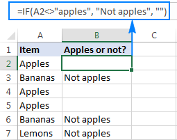
=IF(A2<>"apples", "Not apples", "")
Either way, the formula will produce this result:
If cell contains text: case-sensitive formula
To force your formula to distinguish between uppercase and lowercase characters, use the EXACT function that checks whether two text strings are exactly equal, including the letter case:
=IF(EXACT(A2,"APPLES"), "Yes", "")

You can also input the model text string in some cell (say in C1), fix the cell reference with the $ sign ($C$1), and compare the target cell with that cell:
=IF(EXACT(A2,$C$1), "Yes", "")

If cell contains specific text string (partial match)
We have finished with trivial tasks and move on to more challenging and interesting ones :) To check if a cell contains specific a given character or substring as part of the cell content, you can use one of these formulas:
Formula 1
Working from the inside out, here is what the formula does:
- The SEARCH function searches for a text string, and if the string is found, returns the position of the first character, the #VALUE! error otherwise.
- The ISNUMBER function checks whether SEARCH succeeded or failed. If SEARCH has returned any number, ISNUMBER returns TRUE. If SEARCH results in an error, ISNUMBER returns FALSE.
- Finally, the IF function returns the specified value for cells that have TRUE in the logical test, an empty string ("") otherwise.
Formula 2
Here, the COUNTIF function finds out how many times a certain text appears in a cell. To count partial matches, you place the wildcard character (*) on both sides of the text. If the count is greater than zero, then IF returns the specified value, otherwise - a blank cell.
And now, let's see how this generic formula works in real-life worksheets.
If cell contains certain text, put a value in another cell
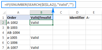
Supposing you have a list of orders in column A and you want to find orders with a specific identifier, say "A-". The task can be accomplished with this formula:
=IF(ISNUMBER(SEARCH("A-", A2)), "Valid", "")
or
=IF(COUNTIF(A2, "*"&"A-"&"*"), "Valid", "")
Instead of hardcoding the string in the formula, you can input it in a separate cell (E1), the reference that cell in your formula:
=IF(ISNUMBER(SEARCH($E$1,A2)), "Valid", "")
or
=IF(COUNTIF(A2, "*"&$E$1&"*"), "Valid", "")
For the formula to work correctly, be sure to lock the address of the cell containing the string with the $ sign (absolute cell reference).
If cell contains specific text, copy it to another column
If you wish to copy the contents of the valid cells somewhere else, simply supply the address of the evaluated cell (A2) in the value_if_true argument:
=IF(ISNUMBER(SEARCH($E$1,A2)),A2,"")
The screenshot below shows the results:

If cell contains specific text: case-sensitive formula
In both of the above examples, the formulas are case-insensitive. In situations when you work with case-sensitive data, use the FIND function instead of SEARCH to distinguish the character case.
For example, the following formula will identify only orders with the uppercase "A-" ignoring lowercase "a-".
=IF(ISNUMBER(FIND("A-",A2)),"Valid","")

If cell contains, then return value – multiple conditions
A single ‘if cell contains’ statement is easy, right? But what if you need to check multiple conditions in the same formula and return different results? That is, if a cell contains some text, then return something, if it contains another text, then return something else, and so on.
To evaluate multiple conditions in a cell, you can use nested "if cell contains" statements. This allows you to create a chain of checks, with each condition leading to a specific result. Here are two generic formulas to achieve this:
Formula 1
Use the COUNTIF function to count how many times a certain text appears in a cell. If the count is greater than zero, then return the corresponding value. Otherwise, check the next condition.
Formula 2
Use the SEARCH function to find the position of a certain text in a cell. If the position is a number, then return the corresponding value. Otherwise, check the next condition.
For example, to checks if cell A2 contains "apple", "banana" or "lemon" and return the corresponding name of the fruit in cell B3, you can use one of these formulas:
=IF(COUNTIF(A2, "*apple*"), "Apple", IF(COUNTIF(A2, "*Banana*"), "Banana", IF(COUNTIF(A2, "*lemon*"), "Lemon", "")))
=IF(ISNUMBER(SEARCH("apple", A2)), "Apple", IF(ISNUMBER(SEARCH("banana", A2)), "Banana", IF(ISNUMBER(SEARCH("lemon", A2)), "Lemon", "")))
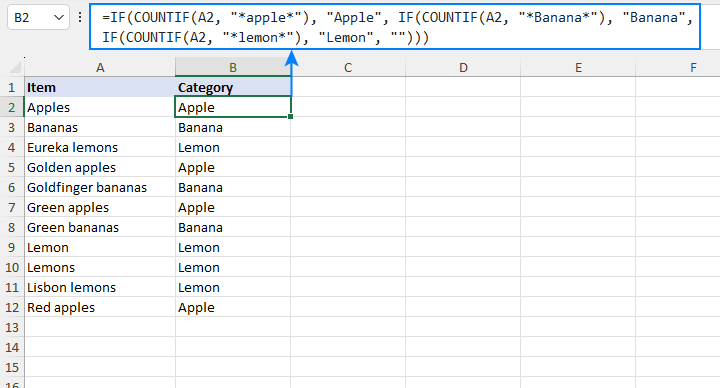
To fit your specific needs, you can extend the chain of conditions as necessary to handle more cases.
If cell contains one of many text strings (OR logic)
To identify cells containing at least one of many things you are searching for, use one of the following formulas.
IF OR ISNUMBER SEARCH formula
The most obvious approach would be to check for each substring individually and have the OR function return TRUE in the logical test of the IF formula if at least one substring is found:
Supposing you have a list of SKUs in column A and you want to find those that include either "dress" or "skirt". You can have it done by using this formula:
=IF(OR(ISNUMBER(SEARCH("dress",A2)),ISNUMBER(SEARCH("skirt",A2))),"Valid ","")
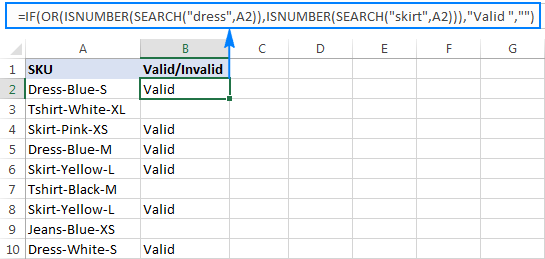
The formula works pretty well for a couple of items, but it's certainly not the way to go if you want to check for many things. In this case, a better approach would be using the SUMPRODUCT function as shown in the next example.
SUMPRODUCT ISNUMBER SEARCH formula
If you are dealing with multiple text strings, searching for each string individually would make your formula too long and difficult to read. A more elegant solution would be embedding the ISNUMBER SEARCH combination into the SUMPRODUCT function, and see if the result is greater than zero:
For example, to find out if A2 contains any of the words input in cells D2:D4, use this formula:
=SUMPRODUCT(--ISNUMBER(SEARCH($D$2:$D$4,A2)))>0
Alternatively, you can create a named range containing the strings to search for, or supply the words directly in the formula:
=SUMPRODUCT(--ISNUMBER(SEARCH({"dress","skirt","jeans"},A2)))>0
Either way, the result will be similar to this:
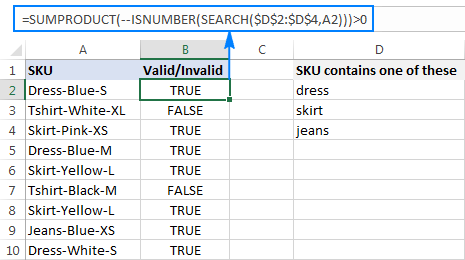
To make the output more user-friendly, you can nest the above formula into the IF function and return your own text instead of the TRUE/FALSE values:
=IF(SUMPRODUCT(--ISNUMBER(SEARCH($D$2:$D$4,A2)))>0, "Valid", "")

How this formula works
At the core, you use ISNUMBER together with SEARCH as explained in the previous example. In this case, the search results are represented in the form of an array like {TRUE;FALSE;FALSE}. If a cell contains at least one of the specified substrings, there will be TRUE in the array. The double unary operator (--) coerces the TRUE / FALSE values to 1 and 0, respectively, and delivers an array like {1;0;0}. Finally, the SUMPRODUCT function adds up the numbers, and we pick out cells where the result is greater than zero.
If cell contains several strings (AND logic)
In situations when you want to find cells containing all of the specified text strings, use the already familiar ISNUMBER SEARCH combination together with IF AND:
For example, you can find SKUs containing both "dress" and "blue" with this formula:
=IF(AND(ISNUMBER(SEARCH("dress",A2)),ISNUMBER(SEARCH("blue",A2))),"Valid ","")
Or, you can type the strings in separate cells and reference those cells in your formula:
=IF(AND(ISNUMBER(SEARCH($D$2,A2)),ISNUMBER(SEARCH($E$2,A2))),"Valid ","")

As an alternative solution, you can count the occurrences of each string and check if each count is greater than zero:
=IF(AND(COUNTIF(A2,"*dress*")>0,COUNTIF(A2,"*blue*")>0),"Valid","")
The result will be exactly like shown in the screenshot above.
How to return different results based on cell value
In case you want to compare each cell in the target column against another list of items and return a different value for each match, use one of the following approaches.
Nested IFs
The logic of the nested IF formula is as simple as this: you use a separate IF function to test each condition, and return different values depending on the results of those tests.
Supposing you have a list of items in column A and you want to have their abbreviations in column B. To have it done, use the following formula:
=IF(A2="apple", "Ap", IF(A2="avocado", "Av", IF(A2="banana", "B", IF(A2="lemon", "L", ""))))

For full details about nested IF's syntax and logic, please see Excel nested IF - multiple conditions in a single formula.
Lookup formula
If you are looking for a more compact and better understandable formula, use the LOOKUP function with lookup and return values supplied as vertical array constants:
For accurate results, be sure to list the lookup values in alphabetical order, from A to Z.
=LOOKUP(A2,{"apple";"avocado";"banana";"lemon"},{"Ap";"Av";"B";"L"})

For more information, please see Lookup formula as an alternative to nested IFs.
Vlookup formula
When working with a variable data set, it may be more convenient to input a list of matches in separate cells and retrieve them by using a Vlookup formula, e.g.:
=VLOOKUP(A2, $D$2:$E$5, 2,FALSE )

For more information, please see Excel VLOOKUP tutorial for beginners.
This is how you check if a cell contains any value or specific text in Excel. Next week, we are going to continue looking at Excel's If cell contains formulas and learn how to count or sum relevant cells, copy or remove entire rows containing those cells, and more. Please stay tuned!
Practice workbook
Excel If Cell Contains - formula examples (.xlsx file)
Latest comments
I am trying to search a number of rows for a specific text "I48.0" and if it is found, would like a separate column to either put 1 or 0 if it is found indicating yes or no. Is there a way anybody can help me do this please? I am lost.
Hello Shawn!
If you want to find a substring in the text, you can use the SEARCH or FIND function. For example:
=ISNUMBER(SEARCH("I48.0",A1))
If the substring is found, the formula will return TRUE. Read more: Excel FIND and SEARCH functions with formula examples.
You can also find useful information in this article: Excel formula to count cells with certain text (exact and partial match).
=COUNTIF(A1,"*"&"I48.0"&"*")>0
To search across more than one row, you can use the range of cells in the formula:
=COUNTIF(A1:A10,"*"&"I48.0"&"*")>0
I am trying to set the value in column D to read “Complete” if there is any text at all in the same row in Column G. I have tried using this guide and I’m not having any success. What’s wrong with my formula?
=IF(G2””,”Complete”,””)
Hello Tori!
You can find the answer to your question in this article: Excel ISBLANK function to check if cell is empty or not. The formula might look like this:
=IF(ISBLANK(G2), "Complete", "")
I need to post a 1 in the subject cell, if another cell contains an A or a B (there may be other letters). I need to post a -1 in the subject cell if the other cell contains a D or an F. The subject cell remains blank if there is not an A, B, D, or F in the other cell. Thanks for any help.
Hello Jerry!
You can use the SEARCH function to search for a letter within a string of text. ISNUMBER function converts the result of the search to True or False. A double minus shows this as 0 or 1. The IF function returns the desired result if the sum of the results is greater than 0.
=IF(SUM(--ISNUMBER(SEARCH({"A","B"},A1))),1, IF(SUM(--ISNUMBER(SEARCH({"D","F"},A1))),-1,""))
I need help displaying a row which contains a particular value in a fresh sheet.
Hi! You can filter one or more rows by condition and display them in a new location using FILTER function.
You can find the examples and detailed instructions here: Excel FILTER function - dynamic filtering with formulas.
Hi, I am trying to use a easy "if" formula and something is not working. I have seen different options already.
So I have a cell with a number X which means the quantity I have in stock. Then I have another cell with the minimum quantity I should have (Y) and another cell with the maximum quantity I am allowed to order for stocking (Z). So I do IF (=IF(Y>X;Z-X;"No need"). This formula is plotted in a final cell to see the result but I always see "No need" text instead of any value when testing it.
I see everywhere using comas (,) but I can't, I am forced to use dot coma (;).
Could you please help me?
Thanks in advance.
Hello Antonio!
If I understood the question correctly, to calculate how many units you can order, try this formula:
=IF(Y1>X1,MIN(Z1,Y1-X1),"No need")
MIN function determines that you can order no more than the maximum quantity that you are allowed to order.
I need help to make a formula - IF the cell is not blank, THEN add the date into another cell. However I want the date to not change. Ie I want to be able to track when text was added to the first cell. Thanks.
Hello Kathryn!
If I understand your task correctly, this guide may be helpful: How to insert today date & current time as unchangeable time stamp
The second option is to use VBA to write the current date and time to the cell.
I need formula where if i need to match a specific text, across multiple cells and if any of the cells match i need return the complete value from that cell.
Hi! You can use one of these instructions: XLOOKUP with partial match (wildcards) or VLOOKUP formula with wildcard or MATCH formula with wildcards. Use MATCH function with wildcards in INDEX MATCH formula.
Hi
I need a formula that reads a date and then moves the data of the row into a new sheet
(schedule via excel)
example if column A has 2.5.2024 move row B to sheet 2
What type of formula do I require?
Hi! If I understand the question correctly, you can search the column for the correct value and extract the corresponding row using INDEX MATCH functions. To extract not just one value, but the entire string from a range, use this instruction: Get all values in a row or column. You can correctly create references to another worksheet as described here: Excel reference to another sheet or workbook (external reference).
I hope it’ll be helpful. If this is not what you wanted, please describe the problem in more detail.
I am trying to identify the column # of a cell within a range that contains 2 different strings of text (ordered if necessary), but those are not the only strings within the cell.
e.g. A1 = string 1, string 2, string 3; A2 = string 1, string 4, string 5; A3 = string 3, string 4, string 6
I would like the formula to look at the range A1:A3 and return the position of the cell with string 1 and string 5. As noted above it can be written so they are ordered or unordered, if one is easier than the other.
Hi! If I understand the question correctly, you can determine the position of the cell that has the text strings "string 1" and "string 5" using the MATCH formula. For example:
=MATCH(1,ISNUMBER(SEARCH("string 1",A1:A3)) * ISNUMBER(SEARCH("string 5",A1:A3)),0)
For more information, please read: How to find substring in Excel
I have a sheet with a list of clients and a list of the companies they work for. Is there a way to say if the cell is equal to a company name to then show the employee name on a separate sheet??
Hi! When you want to find a value and get its corresponding value from another column, use these guidelines and examples: Excel VLOOKUP function tutorial with formula examples and INDEX & MATCH in Excel - better alternative to VLOOKUP.
let say i have a cell that contain "Monday morning, tuesday morning" but by using the if function who do i only say yes to one of them which is Monday?
Hi! To determine a partial text match, try this formula:
=IF(ISNUMBER(SEARCH("Monday",A1)),"Yes","")
For more information, please read: How to find substring in Excel
Hi, I have a large set of data with numerous columns, I need a formula that will search if any cells in a row contain a certain key word, if so, I want it to return the FULL contents of that cell.
Example, say I have in row 2, A2 (Star), A3 ($56), A4 (Changed Sales Rep), A5 (3/4/23 updated to cancelled), a6 (Project Name)
And I want the formula to search for 'Cancelled' and return everything in the cell, in this case it would be cell A5 and the return should be '3/4/23 updated to cancelled'
I essentially have a ton of terrible data outputted that cannot easily be delimeted and I need to find the date tied to any substring within the cells that contain the word cancelled.
Thanks in advance.
Hi! Use the INDEX MATCH formula to get a cell with a partial text match. For more information, please read: How to find substring in Excel
Try this formula:
=INDEX(A1:A10,MATCH(TRUE,ISNUMBER(SEARCH("Cancelled",A1:A10)),0))
I hope it’ll be helpful.
I'm trying to figure out how to get column c cells which contain various number .ie 20227, 208566, I want column d cells to look for a specific number in C and fill D with the value in A i.e shoe, house etc
Hi! If I understand your task correctly, to find a value in a column and get its corresponding value from another column, this article may be helpful: INDEX & MATCH in Excel.
Hi,
Please help provide the formula if a range of cells contain the letters BR, then I would like the sum of another range of cells of just containing BR to return the value, thank you.
Hello!
To find the sum of the cells by condition, try using the SUMIF function. I hope it’ll be helpful. If this is not what you wanted, please describe the problem in more detail.
Hello, I would like to seek help. If a cell has a text value: then perform another formula else blank
Hi!
To check if a value is text, use the Excel IF ISTEXT formula.
Hi Alexander,
I been going crazy trying to get this formula, if you could help me that me very appreciated.
What I am trying to do is
(b1+b2)/2 if b1 or b2 aren't entered don't divide just give me the number that was entered in b1 or b2
Thank you in advance
Hello!
Here is the article that may be helpful to you: Excel IF statement with multiple AND/OR conditions.
=IF(OR(B1="",B2=""),IF(B1="",B2,B1),(B1+B2)/2)
This should solve your task.
Hello
I have an incident where Students are graded in a subject per week from week one to week 16. where each week is in its own column from Column B to Column P. where I grade each student with words "Passed" and "Excelled". I'm crediting their overall performance in another sheet which fetches from my primary sheet and I would like help with an excel function that searches for a word "excelled" in any week from week one to 16 and returns "promoted" if it finds the word "excelled" any where. Thanks!
Hello!
To search for values in the desired line, I recommend using such a formula:
=SUMPRODUCT(--(A2:A20=N1)*(B2:P20= "Excelled"))
N1 - name.
If the formula returns the number more than 0, then the desired word is found for this student.
I hope it’ll be helpful.
Hello
Is there a way of using the below formula, but rather than have it search for the specific text only within a cell, it can search a sentence containing "apple" or "banana" etc then return the value based on the sentence content? I need the formula to be able to search for multiple fruits and return the value in another cell depending on what fruit it found within the sentence.
For example, cell A1 contains the sentence, "Mr Smith ate an apple".
cell B1 should then return Apple. However, if cell A1 contained, "Mr Smith ate a banana", cell B2 should return "Banana".
=IF(A2="apple", "Ap", IF(A2="avocado", "Av", IF(A2="banana", "B", IF(A2="lemon", "L", ""))))
Hope this makes sense!
Thank you
Hi Rhys,
COUNTIF with wildcards in the criteria works a treat:
=IF(COUNTIF(A2, "*apple*")>0, "Ap", IF(COUNTIF(A2, "*avocado*")>0, "Av", IF(COUNTIF(A2, "*banana*")>0, "B", IF(COUNTIF(A2, "*lemon*")>0, "L", ""))))
HI,
I Have a column, M, named "Qualifications". It contains different strings of Academic qualification data. But I just need to pick the specific qualification. E.g If the string reads " Masters of Education", I just need "Masters" If it reads "Certificate of Secondary Education", I need KCSE, If it reads "Bachelors degree in Medicine", I just need "Bachelors".
Tried using the formula below but didn't work. PLease HELP
=LOOKUP(M2{"*Doctor*";"*Master*";"*Bachelor*";"*Diploma*";"*Secondary*";"*CSE*";"*EACE*";"*Primary*";"*CPE*";"*N/A*"} "PhD";"Masters";"Bachelors";"Diploma";"KCSE";"KCSE";"KCSE";"KCPE";"KCPE";"N/A"})
Teddy:
Wildcards can be used in some functions, but not in others. If you need to use the * in the formula you'll need to use VLOOKUP or an INDEX/MATCH formula.
Here's how to write a nested IF statement for the samples you provided:
=IF(A74="Doctor","PHD", IF(A74="Master","Masters",IF(A74="Bachelor","Bachelors", IF(A74="Secondary","KCSE", IF(A74="Diploma","KCSE", IF(A74="CSE","KCSE", IF(A74="EACE","KCSE", IF(A74="Primary","CPE", IF(A74="N/A","N/A")))))))))
You can use this as the basis for a huge IF/OR statement, but it would get crazy long.
Read the VLOOKUP or INDEX/MATCH articles here on AbleBits and see if that helps.