The tutorial shows how to merge multiple arrays in Excel 365 vertically and horizontally using VSTACK and HSTACK functions.
Combining two or more ranges has traditionally been a daunting task in Excel. Not any longer! The two functions recently introduced in Excel 365, VSTACK and HSTACK, have made the job incredibly easy. Now, merging ranges and arrays, even dynamic ones whose sources are variable in size, is as easy as supplying a couple of range references to a formula.
Excel VSTACK function
The VSTACK function in Excel combines multiple arrays or ranges vertically into a single array. Each subsequent array is appended to the first blank cell at the bottom of the previous array.
Syntax
The VSTACK function takes the following arguments:
Where arrays are cell ranges or arrays to join. Array1 is required; array2 and subsequent ones are optional.
Result
The output of VSTACK is a single array that has as many columns as the largest of the source arrays and as many rows as all of the source arrays combined.
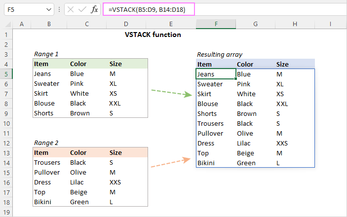
For example, to combine two ranges vertically, the formula is:
=VSTACK(B5:D9, B14:D18)
Excel HSTACK function
The HSTACK function in Excel merges multiple ranges or arrays horizontally into a single array. Each subsequent array is added to the right of the preceding array.
Syntax
The HSTACK function takes the following arguments:
Where arrays are cell ranges or arrays to join. Only array1 is required; additional arrays are optional.
Result
As an output, the HSTACK function returns a single array that has as many columns as all of the source arrays combined and as many rows as the tallest of the source arrays.
For example, to combine two ranges horizontally, the formula is:
=HSTACK(C4:F6, I4:L6)

VSTACK and HSTACK availability
Both functions are only available in Excel for Microsoft 365 (Windows and Mac) and Excel for the web.
VSTACK and HSTACK functions - things to remember
To effectively use the VSTACK and HSTACK functions in your worksheets, here are some key facts to take note of:
- The functions can merge ranges of cells, named ranges, array constants, and dynamic arrays returned by other formulas.
- The formula should be entered just in one cell - the leftmost cell of the destination range. The resulting array automatically spills into as may cells as needed.
- The output is fully dynamic. As soon as any change in the original arrays occurs, the returned array is updated at once.
- To have new data included in the resulting array automatically without updating the formula, you can use Excel tables for source arrays or refer to dynamic arrays as explained in the above-linked examples.
How to combine arrays in Excel - formula examples
With the VSTACK and HSTACK functions, combining ranges in Excel is really easy and straightforward. The below examples will give you some inspiration to get started and show best practices approaches.
Stack arrays horizontally or vertically
Depending on the structure of your original arrays and the layout of your worksheet, you can prefer combining ranges vertically or horizontally.
To merge multiple ranges into a single horizontal stack, use the HSTACK function. In this case, the ranges are stacked next to each other. For instance:
=HSTACK(B3:B7, B12:B16, B21:B25)
To combine multiple ranges into a single vertical stack, utilize the VSTACK function. In this case, the ranges are placed below each other. For example:
=VSTACK(B3:B7, B12:B16, B21:B25)
For better visualization, we are combining ranges including their headers. In real worksheets, you would normally join only data without column headers.

Merge ranges and array constants
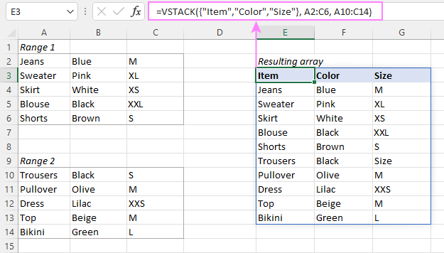
In situations when column headers or some values are missing the original ranges, you can supply the missing data in an array constant directly to the VSTACK or HSTACK function. For example:
=VSTACK({"Item","Color","Size"}, A2:C6, A10:C14)
As a result, you'll get two ranges stacked vertically below each other.
Combine multiple Excel tables into one
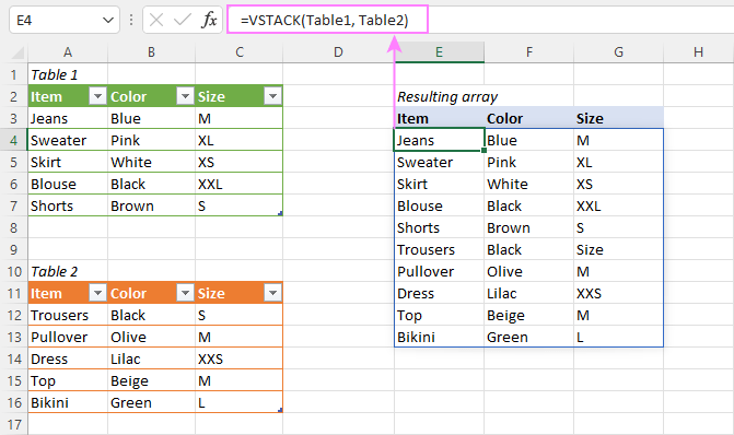
Aside from arrays and ranges, the VSTACK and HSTACK functions can also merge multiple Excel tables into one. Given that Excel tables automatically expand to include new data, this is a perfect solution for data sets of variable size. Simply, supply table references to VSTACK and HSTACK, and you won't have to worry about updating your formulas no matter how many new row/columns of data are added to the source tables.
=VSTACK(Table1, Table2)
Merge dynamic arrays
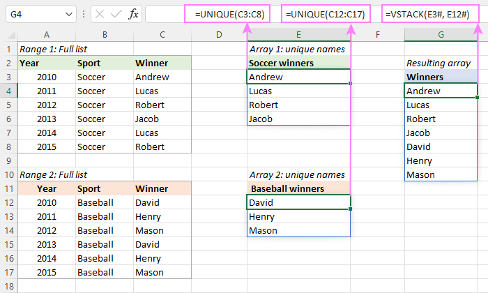
If the arrays you are combining are dynamic, i.e. returned by dynamic array formulas, you can join such arrays by using the spill range operator, which is a hash tag (#) appended to the address of the upper left cell in the spill range.
For example, to combine two arrays generated by the UNIQUE function in the screenshot below, you can use this formula:
=VSTACK(E3#, E12#)
Where E3 is the topmost cell of the first array and E12 is the topmost cell of the second array.
The benefit of this approach is that with any change in the source data, all 3 arrays will be recalculated and updated automatically by Excel.
Handle blanks cells
In case the sources ranges contain empty cells, the returned array will have zeros in the place of blanks. To fix this, you can nest your VSTACK or HSTACK function in the first argument of SUBSTITUTE and tell it to replace zeros with empty strings (""). For example:
=SUBSTITUTE(VSTACK(A3:B7, A12:B16), 0, "")

If your original arrays contain zero values, then substitute empty strings rather than zeros to avoid replacing absolutely all zeros in the returned array. For example:
=SUBSTITUTE(VSTACK(A3:B7, A12:B16), "", "")
Substituting an empty string with an empty string may seem illogical, but it does work. In a stacked array, Excel displays zeroes instead of blanks only for better visualization; in fact those cells are empty.

Combine ranges and remove empty rows
When there are any blank rows or columns in the sources ranges, the resulting array will have zero-filled rows or columns in their place. To eliminate such rows and/or columns, you can filter out blanks with the help of the FILTER function.
The general idea is to supply the VSTACK or HSTACK output to the array argument of the FILTER function and use instruct it to filter non-empty entries (<>"").
Essentially there can be three basic scenarios:
Filter out blanks based on the key column
To filter all rows in which a particular column is not blank, check that specific column. For example, to combine rows that have any value in column A, the formula in D4 is:
=FILTER(VSTACK(A3:B7, A12:B16), VSTACK(A3:A7, A12:A16)<>"")
Remove absolutely blank rows
To remove empty rows that do not have a single value in them, each column should be checked individually. To have it done, in the include argument of the FILTER function, you supply a separate criterion for each column and use the plus sign (+) to test them with the OR logic.
For example, to only remove absolutely blank rows and keep those that have a value in any column, the formula in G4 is:
=FILTER(VSTACK(A3:B7, A12:B16), (VSTACK(A3:A7, A12:A16)<>"")+(VSTACK(B3:B7, B12:B16)<>""))
For more information, please see How to filter with multiple OR criteria.
Eliminate all blanks
To filter out rows that have at least one empty cell in any column, you again check each individual column for non-blanks, but this time test the criteria with the AND logic using the asterisk (*).
For example, to remove rows that have blanks in either column A or B, the formula in E16 is:
=FILTER(VSTACK(A3:B7,A12:B16),(VSTACK(A3:A7,A12:A16)<>"")*(VSTACK(B3:B7,B12:B16)<>""))
For more details, please see How to filter with multiple AND criteria.

Tips:
- Though the VSTACK and HSTACK functions return zeroes instead of empty cells, this is purely for presentation reasons. As there is no data in those cells, we use <>"" for the FILTER criteria. The <>0 criteria will work too.
- To replace zeros with empty strings in the resulting array, use the SUBSTITUTE function as explained in the previous example.
- This approach comes in handy for merging variable arrays that may grow in size as new data is added. Simply, stack more rows/columns than are currently filled with data and filter out the empty ones.
Combine ranges without duplicates
To combine only unique records from two or more ranges, use the stacking functions together with UNIQUE.
For example, to stack ranges B2:E4 and H2:K4 horizontally without duplicates, the formula in C8 is:
=UNIQUE(HSTACK(B2:E4, H2:K4), TRUE)
The logical value TRUE in the 2nd argument of UNIQUE tells the function to compare data across columns, not rows.
As the result, the 2nd occurrence of the year 2017 is left out of the resulting array:

Join and sort arrays at once
When merging huge arrays, as a finishing touch, you may want to sort the output. This is quite easy to do by nesting HSTACK or VSTACK in another dynamic array function - SORT.
In our case, the formula takes this form:
=SORT(HSTACK(B2:E4, H2:K4), 1, 1, TRUE )
Breaking down the formula, this is what we have:
- HSTACK(B2:E4, H2:K4) is the array to sort.
- 1 in the 2nd argument is the sort index, i.e. the array is sorted by the first row (Year).
- 1 in the 3rd argument indicates the ascending sort order.
- TRUE means to sort columns, not rows.

Combining same ranges from multiple sheets - 3D formula
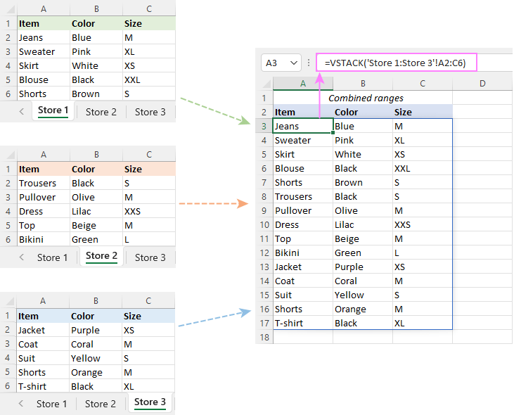
To combine the same range of cells from different worksheets, use a 3D reference in your HSTACK or VSTACK formula.
To make a 3D VSTACK formula for the datasets below, this is what you need to do:
- In the leftmost cell of the destination range (A3), start typing the formula: =VSTACK(
- Click the tab of the first worksheet.
- While holding the Shift key, click the tab of the last worksheet.
- Select the range that you want to combine in all of the sheets.
- Type the closing parenthesis and press the Enter key.
The completed formula will look as follows:
=VSTACK('Store 1:Store 3'!A2:C6)
If your original datasets are likely to expand in future, you can include more rows than are currently populated with data, and then filter out empty rows. For instance:
=FILTER(VSTACK('Store 1:Store 3'!A2:C100), VSTACK('Store 1:Store 3'!A2:A100)<>"")
How to combine arrays of different size without errors
When merging two or more arrays of different size, Excel "expands" smaller array(s) to match the size of the largest one and returns #N/A errors in place of the missing values. To catch and handle those errors, you can use the IFNA function in Excel 2013 and higher or IFERROR in earlier versions.
In the below formula, IFNA is configured to replace #N/A errors with empty strings (""), which look like blank cells to the human eye.
=IFNA(HSTACK(B2:E4, H2:J3), "")

VSTACK and HSTACK not working
If the functions do not work as expected or are not available in your Excel, you are likely to get one of these errors.
#NAME? error
Normally, occurs if the function's name is misspelled, but may also indicate that the function is not available in your Excel version. Please remember that VSTACK and HSTACK are only supported in Excel 365. For more information, see How to fix #NAME error in Excel.
#SPILL! error
Occurs if one or more cells in the spill range are not completely blank. To fix it, just clear the obstructing cells. For more information, please see SPILL! error in Excel: causes and fixes
#N/A error
If one of the source arrays has fewer columns than the largest array, VSTACK returns #N/A errors in the columns where values are missing.
If one of the source arrays has fewer rows than the largest array, HSTACK returns #N/A errors in extra rows.
The solution is to use the IFNA or IFERROR function to replace errors with empty stings or another value of your choice as shown in this example.
That's how to combine arrays in Excel 365 using the VSTACK and HSTACK functions. I thank you for reading and hope to see you on our blog next week!
Practice workbook for download
Stack ranges in Excel – formula examples (.xlsx file)
 by
by
16 comments
How can I select say 2000 arrays to be combined into one? Listing all of them individually becomes a bit difficult, and all of them are of different length too.
Thoughts?
Hi! If your arrays have some distinguishing features by which they can be identified, then you can create and use VBA macro that will select these arrays by the features you specify and combine them
if i have around 3-4 sets of data that i'm bringing by hstack formula and then want to combine using vstack but i need to leave 2 blank rows between each result and i donot know how many rows will be appearing in each result, how can i make it dynamically work to insert blank rows between the hstack results.
Hello Ravali!
To combine named ranges vertically and insert 2 blank rows between them, try this formula:
=VSTACK(
Range1,
MAKEARRAY(2, COLUMNS(Range1), LAMBDA(r,c, "")),
Range2,
MAKEARRAY(2, COLUMNS(Range2), LAMBDA(r,c, "")),
Range3)
Explanation:
VSTACK: Merges ranges vertically.
MAKEARRAY: Creates an array of specified size by filling it with empty strings.
LAMBDA: Function for generating values in an array; in this case returns an empty string for each element.
I hope it’ll be helpful.
Hi, i liked your easy to understand guide, thanks for putting in the work. But in picture three you show that VSTACK can copy the headers with their formating how is this possible? When i do it it copies the text in the header cell but without its formating. Could you please help me fix this. I didn't find any other tutorial that uses VSTACK to list "visual" tables/lists (not real excel tables) underneath eacht other.
Hello Michael!
Unfortunately, Excel VSTACK function does not copy the formatting of the cells it combines into an array. It simply combines values from different ranges into a single column, but the formatting remains the same. In the picture, the cells are highlighted in color for a better understanding of how the function works.
Hello.
this can convert an matrix/table, into array (so I could plot the graph, not 3D).. excellent.
e.g. Hstack( a1:a3, b1:b3, c1c3)
.
1 2 3
4 5 6 to 1 2 3 4 5 6 7 8 9
7 8 9
Can the cell names (e.g. a1:a3) be variables ? Or otherwise cope with one matrix dimension being variable (Y in this case)...
I have a matrix of data that is always 8 across, but may be 64, 500, or 1000 deep, that I need to make into single array (to plot a graph).
Many thanks
Hi! Combine all values into a text string using the TEXTJOIN function. Then split the text string into columns using TEXTSPLIT function.
=TEXTSPLIT(TEXTJOIN(",",,A1:C3),",")
Hope this is what you need.
If i have the array in below format
col 1 col 2
------ xxxxx
------ xxxxx
------ xxxxx
but i want the format to look like
col 1 ------
col 1 ------
col 1 ------
col 1 ------
col 2 xxxxx
col 2 xxxxx
col 2 xxxxx
col 2 xxxxx
how do i do this? pls help
Hi! You can use the Create Cards tool. Set the options "My table has 1 header row", "Number of colunns" - 1, "Add Header".
It is available as a part of our Ultimate Suite for Excel that you can install in a trial mode and check how it works for free.
I hope it’ll be helpful. If something is still unclear, please feel free to ask.
Great stuff your blogs... thanks a lot.
I combine dynamic web scraped tables (up to 20) which sometimes/often are empty or do not exist - so I get an #NA error when empty or not existant; see below
Table 1 with entries: XXXX XXXX Corporation $27.56 $0.50 -2.54% 362,835 287,937 3.465B 15.39 (many rows)
Table 2 not existing (or empty): #N/A #N/A #N/A #N/A #N/A #N/A #N/A #N/A (one row)
The formula is:
=VSTACK(IFERROR(FILTER($O$3:$W$102,(LEFT($N$3:$N$102,2)"LP")*($N$3:$N$102"")),""),IFERROR(FILTER($AC$3:$AK$102,(LEFT($AB$3:$AB$102,2)"LP")*($AB$3:$AB$102"")),""))
Without the IFERROR lines the calculation does not proceed (empty array).
Is there any way to show blank cells in the stack (not #NA) or to avoid them totally with another filter command?
Thanks for your kind consideration...
Hello!
I cannot check or correct your formula as it is written with errors. I recommend that you try using the third argument of the FILTER function: [if_empty] - the value to return when no entries meet the criteria. I hope my advice will help you solve your task.
Hi this is very informative!
However, I have a table(raw_0) which is a source for my query and I have two separate sheets(raw_1 and raw_2) where I input my raw data. I input the vstack formula on my table source(raw_0) but it's a table so there's spilling error.
Is there any workaround?
Hi Kevin,
Regrettably, dynamic array functions (including VSTACK and HSTACK) do not work from within Excel tables, only within regular ranges.
Today when I was writing a formula as usual with vlookup I realized that there is one more formula on the screen. I noticed immediately that it was new so I looked it up on google and found this page.
You have shown an awesome explanation and examples.
I will digest it with practice.
Thanks
Hi!
Thank you for your feedback. Today we have published an article about one more new function. Hopefully, you will find it helpful too:
Excel TOCOL function - convert range to single column