The tutorial shows how to insert table in Excel and explains the advantages of doing so. You will find a number of nifty features such as calculated columns, total row and structured references. You will also gain understanding of Excel table functions and formulas, learn how to convert table to range or remove table formatting.
Table is one of the most powerful Excel features that is often overlooked or underestimated. You may get along without tables just fine until you stumble upon them. And then you realize you've been missing an awesome tool that could save much of your time and make your life a lot easier.
Converting data to a table can spare you the headache of creating dynamic named ranges, updating formula references, copying formulas across columns, formatting, filtering and sorting your data. Microsoft Excel will take care of all this stuff automatically.
What is a table in Excel?
Excel table is a named object that allows you to manage its contents independently from the rest of the worksheet data. Tables were introduced in Excel 2007 as in improved version of Excel 2003 List feature, and are available in all subsequent versions of Excel 2010 through 365.
Excel tables provide an array of features to effectively analyze and manage data such as calculated columns, total row, auto-filter and sort options, automatic expansion of a table, and more.
Typically, a table contains related data that are entered in a series of rows and columns, though it can consist of a single row and/or column. The screenshot below shows a difference between a usual range and a table:

Note. An Excel table should not be confused with a data table, which is part of the What-If Analysis suite that allows calculating multiple results.
How to make a table in Excel
Sometimes, when people enter related data in a worksheet, they refer to that data as a "table", which is technically incorrect. To convert a range of cells into a table, you need to explicitly format it as such. As is often the case in Excel, there is more than one way to do the same thing.
3 ways to create a table in Excel
To insert a table in Excel, organize your data in rows and columns, click any single cell within your data set, and do any of the following:
- On the Insert tab, in the Tables group, click Table. This will insert a table with the default style.

- On the Home tab, in the Styles group, click Format as Table, and select one of the predefined table styles.
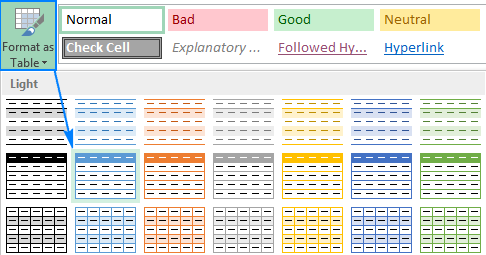
- If you prefer working from the keyboard rather than using a mouse, the fastest way to create a table is pressing the Excel Table shortcut: Ctrl+T
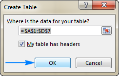
Whatever method you choose, Microsoft Excel automatically selects the entire block of cells. You verify if the range is selected correctly, check or uncheck the My table has headers option, and click OK.
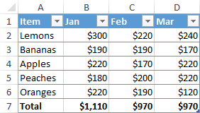
As the result, a nicely formatted table is created in your worksheet. At first sight, it may look like a normal range with the filter buttons in the header row, but there is much more to it!
Notes:
- If you want to manage several independent data sets, you can make more than one table in the same sheet.
- It is not possible to insert a table in a shared file because the table functionality is not supported in shared workbooks.
10 most useful features of Excel tables
As already mentioned, Excel tables offer a number of advantages over normal data ranges. So, why don't you benefit from the powerful features that are now only a button click away?
1. Integrated sorting and filtering options
Usually it takes a few steps to sort and filter data in a worksheet. In tables, filter arrows are automatically added in the header row and enable you to use various text and number filters, sort in ascending or descending order, by color, or create a custom sort order.
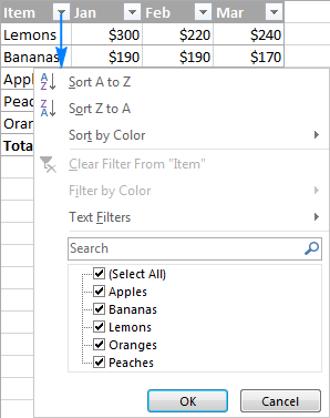
If you don't plan to filter or sort your data, you can easily hide the filter arrows by going to the Design tab > Table Style Options group, and unchecking the Filter Button box.
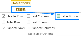
Or, you can toggle between hiding and showing the filter arrows with the Shift+Ctrl+L shortcut.
Additionally, in Excel 2013 and higher, you can create a slicer to filter the table data quickly and easily.
2. Column headings are visible while scrolling
When you are working with a large table that does not fit on a screen, the header row always remains visible when you scroll down. If this doesn't work for you, just be sure to select any cell inside the table before scrolling.
3. Easy formatting (Excel table styles)
A newly created table is already formatted with banded rows, borders, shading, and so on. If you don't like the default table format, you can easily change it by selecting from 50+ predefined styles available in the Table Styles gallery on the Design tab.

Apart from changing table styles, the Design tab lets you turn the following table elements on or off:
- Header row - displays column headers that remain visible when you scroll the table data.
- Total row - adds the totals row at the end of the table with a number of predefined functions to choose form.
- Banded rows and banded columns - display alternate row or column colors.
- First column and last column - display special formatting for the first and last column of the table.
- Filter button - shows or hides filter arrows in the header row.
The screenshot below shows the default Table Style Options:
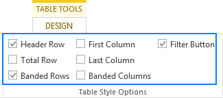
Table Styles tips:
- If the Design tab has disappeared from your workbook, just click any cell within your table and it will show up again.
- To set a certain style as the default table style in a workbook, right-click that style in the Excel Table Styles gallery and select Set As Default.
- To remove table formatting, on the Design tab, in the Table Styles group, click the More button
 in the bottom-right corner, and then click Clear underneath the table style thumbnails. For full details, see How to clear table formatting in Excel.
For more information, please see How to use Excel table styles.
4. Automatic table expansion to include new data
Usually, adding more rows or columns to a worksheet means more formatting and reformatting. Not if you've organized your data in a table! When you type anything next to a table, Excel assumes you want to add a new entry to it and expands the table to include that entry.

As you can see in the screenshot above, the table formatting is adjusted for the newly added row and column, and alternate row shading (banded rows) is kept in place. But it's not just the table formatting that is extended, the table functions and formulas are applied to the new data too!
In other words, whenever you draw a table in Excel, it is a "dynamic table" by nature, and like a dynamic named range it expands automatically to accommodate new values.
To undo the table expansion, click the Undo button ![]() on the Quick Access Toolbar, or press Ctrl+Z like you usually do to revert the latest changes.
on the Quick Access Toolbar, or press Ctrl+Z like you usually do to revert the latest changes.
5. Quick totals (total row)
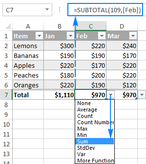
To quickly total the data in your table, display the totals row at the end of the table, and then select the required function from the drop-down list.
To add a total row to your table, right click any cell within the table, point to Table, and click Totals Row.
Or, go to the Design tab > Table Style Options group, and select the Total Row box:

Either way, the total row appears at the end of your table. You choose the desired function for each total row cell, and a corresponding formula is entered in the cell automatically:
Total Row tips:
- Excel table functions are not limited to the functions in the drop-down list. You can enter any function you want in any total row cell by clicking More Functions in the dropdown list or entering a formula directly in the cell.
- Total row inserts the SUBTOTAL function that calculates values only in visible cells and leaves out hidden (filtered out) cells. If you want to total data in visible and invisible rows, enter a corresponding formula manually such as SUM, COUNT, AVERAGE, etc.
6. Calculating table data with ease (calculated columns)
Another great benefit of an Excel table is that it lets you calculate the entire column by entering a formula in a single cell.
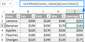
For example, to create a calculated column in our sample table, enter an Average formula in cell E2:

As soon as you click Enter, the formula is immediately copied to other cells in the column and properly adjusted for each row in the table:
Calculated Column tips:
- If a calculated column is not created in your table, make sure the Fill formulas in tables to create calculated columns option is turned on in your Excel. To check this, click File > Options, select Proofing in the left pane, click the AutoCorrect Options button, and switch to AutoFormat As You Type tab.
- Entering a formula in a cell that already contains data does not create a calculated column. In this case, the AutoCorrect Options button appears (like in the screenshot below) and lets you overwrite the data in the entire column so that a calculated column is created.
- You can quickly undo a calculated column by clicking the Undo Calculated Column in AutoCorrect Options, or clicking the Undo button on the Quick Access toolbar.

7. Easy-to-understand table formulas (structured references)
An indisputable advantage of tables is the ability to create dynamic and easy-to-read formulas with structured references, which use table and column names instead of regular cell addresses.
For example, this formula finds an average of all the values in columns Jan through Mar in the Sales_table:
=AVERAGE(Sales_table[@[Jan]:[Mar]])
The beauty of structured references is that, firstly, there are created automatically by Excel without you having to learn their special syntax, and secondly, they adjust automatically when data is added or removed from a table, so you don't have to worry about updating the references manually.
For more information, please see Structured reference in Excel tables.
8. One-click data selection
You can select cells and ranges in a table with the mouse like you normally do. You can also select table rows and columns in a click.
9. Dynamic charts
When you create a chart based on a table, the chart updates automatically as you edit the table data. Once a new row or column is added to the table, the graph dynamically expands to take the new data in. When you delete some data in the table, Excel removes it from the chart straight away. Automatic adjustment of a chart source range is an extremely useful feature when working with data sets that frequently expand or contract.
10. Printing only the table
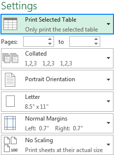
If you want to print just the table and leave out other stuff on the worksheet, select any sell within your table and press Ctrl+P or click File > Print. The Print Selected Table option will get selected automatically without you having to adjust any print settings:
How to manage data in an Excel table
Now that you know how to make a table in Excel and use its main features, I encourage you to invest a couple more minutes and learn a few more useful tips and tricks.
How to convert a table to a range
If you want to remove a table without losing the table data or table formatting, go to the Design tab > Tools group, and click Convert to Range.
Or, right-click anywhere within the table, and select Table > Convert to Range.
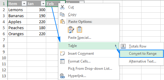
This will delete a table but keep all data and formats intact. Excel will also take care of the table formulas and change the structured references to normal cell references.
For more information, please see How to convert Excel table to normal range .
How to add or remove table rows and columns
As you already know, the easiest way to add a new row or column to a table is type any value in any cell that is directly below the table, or type something in any cell to the right of the table.
If the Totals row is turned off, you can add a new row by selecting the bottom right cell in the table and pressing the Tab key (like you would do when working with Microsoft Word tables).
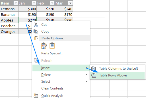
To insert a new row or column inside a table, use the Insert options on the Home tab > Cells group. Or, right-click a cell above which you want to insert a row, and then click Insert > Table Rows Above; to insert a new column, click Table Columns to the Left.
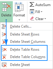
To delete rows or columns, right-click any cell in the row or column you want to remove, select Delete, and then choose either Table Rows or Table Columns. Or, click the arrow next to Delete on the Home tab, in the Cells group, and select the required option:
How to select rows and columns in a table
Generally, you can select data in your Excel table in the usual way using the mouse. In addition, you can use the following one-click selection tips.
Selecting a table column or row
Move the mouse point to the top edge of the column header or the left border of the table row until the pointer changes to a black pointing arrow. Clicking that arrow once selects only the data area in the column; clicking it twice includes the column header and total row in the selection like shown in the following screenshot:

Tip. If the whole worksheet column or row gets selected rather than a table column / row, move the mouse pointer on the border of the table column header or table row so that the column letter or row number is not highlighted.
Alternatively, you can use the following shortcuts:
- To select a table column, click any cell within the column, and press Ctrl+Space once to select only the column data; and twice to select the entire column including the header and total row.
- To select a table row, click the first cell in the row, and then press Ctrl+Shift+right arrow.
How to copy /paste a column within Excel table
Excel tables were designed to make various tasks easier, but one simple action often confuses users – copying the data from one column to another within the same table. Attempting the familiar copy-paste technique may result in this error message:

The error message precisely identifies the issue: a selection that includes cells inside and below a table cannot be copied into the table. Simply put, to copy table columns, it's essential to only select data within the table itself, rather than entire columns in the worksheet.
To copy table columns effectively, follow these steps:
- Select the column. For the column you want to copy, do one of the following:
- Move your mouse pointer to the top edge of the column header until it transforms into a black pointing arrow. Click the arrow once to select only the data rows; click twice to select the table column, including the header and total row.
- Alternatively, click any cell within the column and press Ctrl + Space once to select only the column data; press it twice to select the entire column, including the header.

Note. Ensure the column letter is not highlighted when clicking the pointing arrow with the mouse, as this selects the entire worksheet column. To avoid this, move the mouse pointer slightly down on the border of the column header.
- Copy the selected column. Use the Ctrl + C shortcut to copy the selected column, or right-click and choose Copy from the context menu.

- Paste the copied column. Select the top cell in the destination column and press Ctrl + V to paste the copied data. Or right-click and select Paste from the context menu.

Done! By following these steps, you can efficiently copy columns within an Excel table without errors.
How to resize an Excel table
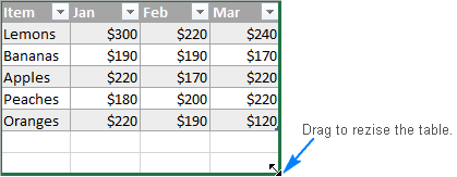
To resize a table, i.e. include new rows or columns to the table or exclude some of the existing rows or columns, drag the triangular resize handle at the bottom-right corner of the table upwards, downwards, to the right or to the left:
Selecting an entire table
To select the table data area, click the upper-left corner of the table, the mouse pointer will change to a south-east pointing arrow like in the screenshot below. To select the entire table, including the table headers and total row, click the arrow twice.

Another way to select the table data is to click any cell within a table, and then press CTRL+A. To select the entire table, including the headers and totals row, press CTRL+A twice.
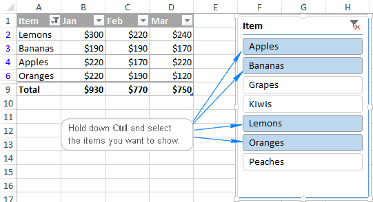
Insert a slicer to filter table data in the visual way
In Excel 2010, it is possible to create slicers for pivot tables only. In newer versions, slicers can also be used for filtering table data.
To add a slicer for your Excel table, just do the following:
- Go to the Design tab > Tools group, and click the Insert Slicer button.
- In the Insert Slicers dialog box, check the boxes for the columns that you want to create slicers for.
- Click OK.
As the result, one or more slicers will appear in your worksheet, and you simply click the items you want to show in your table.
Tip. To display more than one item, hold down the Ctrl key while picking the items.
How to name a table in Excel
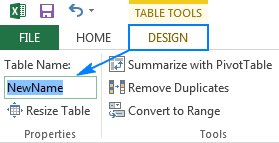
When you create a table in Excel, it is given a default name such as Table 1, Table 2, etc. In many situations, the default names are fine, but sometimes you may want to give your table a more meaningful name, for example, to make the table formulas easier to understand. Changing the table tame is as easy as it can possibly be.
To rename an Excel table:
- Select any cell within the table.
- On the Design tab, in the Properties group, type a new name in the Table Name box.
- Press Enter.
That's all there is to it!
How to remove duplicates from a table
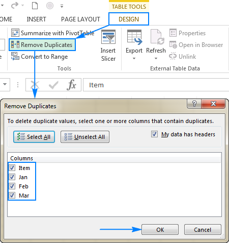
This is another awesome feature of Excel tables that many people are totally unaware of. To delete duplicate rows in your table, just do the following:
- Got to the Design tab > Tools group, and click Remove Duplicates.
- In the Remove Duplicates dialog box, select the columns that may contain duplicates.
- Click OK.
Done!
Tip. If you have inadvertently removed the data that should be kept, click the Undo button or press Ctrl+Z to restore the deleted records.
This tutorial is just a quick overview of the main Excel table features. Just give them a try, and you will find new uses of tables in your daily work and discover new fascinating capabilities. I thank you for reading and look forward to seeing you on our blog next week!
 by
by
15 comments
Regarding Comment Number 1
Thanks. I have been through the guide: Excel Paste Special: copy values, comments, column's width and more.
I may have missed this, but I cannot find any reference in the guide as to how one can copy and paste a column to another column within the same Excel Table. I can do this from within a Range, but not within a Table. I would appreciate some more advice. Thanks.
Hi Joseph,
It's an interesting question! We've never thought that copying columns within a table may cause any problems until we attempted it using the traditional method :) When it comes to copying table columns, it's crucial to remember one key point: you should only select data within the table itself, rather than entire columns in the worksheet. As long as this condition is met, the familiar copy-pasting technique works without any issues.
We've added a separate section to this tutorial outlining the steps: How to copy a column within Excel table. Hope this answers your question.
Is it possible to copy a Column and paste this to another Column in the same Table in Excel?
Thanks
Hi!
I recommend reading this guide: Excel Paste Special: copy values, comments, column's width and more. You can copy and paste the column.
=XLOOKUP(C7,Table5[[#All],[Product]],Table5[[#All],[N]])
I want to change the Table5 part by making use of a cell reference say A7
What is the correct format to change the Table5 part, so that it can lookup in another Table?
Hello!
I recommend reading this guide: Structured references in Excel tables
Hi, how can I remove a table (definition), withaout affecting data.
Hi Kostis,
Right-click any cell in your table, and then choose Table > Convert to Range in the context menu. This will convert the table back to a normal range keeping all the data.
Can you let me know how to coppy data of a column to another column in an Excel table? coppying and pasting data of a column into another in table is similar to coppying and pasting data of a column into another in a normal range?
Hi Sunny,
Yes, copying data from one column into another in a table is similar to copy-pasting data in a normal range, except that you should only select data within a table. When attempting to copy entire worksheet columns, an error occurs.
I want to learn Excel formula plz link me
Hi Washin,
Please check out this tutorial: Basic Excel formulas & functions with examples.
Hi, how do you remove the borders from an excel table? The normal excel borders button does not do the trick for me.
In addition to Doug's response:
You can also create your custom table style without borders:
1. On the Design tab, in the Table Styles group, click the More button.
2. Underneath the table style templates, click New Table style.
3. Under Table Elements, select Whole Table, and click the Format button.
4. Switch to the Border tab, and select None.
For more information, please see How to create a custom table style in Excel.
Benjamin:
AbleBits has this to say about removing formatting from a table:
How to remove table formatting
If you want to keep all features of an Excel table and remove only the formatting such as banded rows, shading and borders, you can clear the table format in this way:
Select any cell in the table.
On the Design tab, in the Table Styles group, click the More button.
Underneath the table style templates, click Clear.
Beyond that I don't know another way. As you have discovered, tables are not regular cells.