This tutorial will teach you a few quick ways to randomly select names, numbers or any other data. You will also learn how to get a random sample without duplicates and how to randomly select a specified number or percentage of cells, rows or columns in a mouse click.
Whether you do market research for a new product launch or evaluating the results of your marketing campaign, it is important that you use an unbiased sample of data for your analysis. And the easiest way to achieve this is to get random selection in Excel.
What is random sample?
Before discussing sampling techniques, let's provide a bit of background information about random selection and when you might want to use it.
In probability theory and statistics, a random sample is a subset of data selected from a larger data set, aka population. Each element of a random sample is chosen entirely by chance and has an equal probability of being selected. Why would you need one? Basically, to get a non-biased representation of the total population.
For example, you want to conduct a little survey among your customers. Obviously, it would be unwise to send out a questionnaire to each single person in your multi-thousand database. So, whom do your survey? Will that be 100 newest customers, or the first 100 customers listed alphabetically, or 100 people with the shortest names? None of these approaches fit your needs because they are innately biased. To get an impartial sample where everyone carries an equal opportunity of being chosen, do a random selection by using one of the methods described below.
Excel random selection with formulas
There's no built-in function to randomly pick cells in Excel, but you can use one of the functions to generate random numbers as a workaround. These probably cannot be called simple intuitive formulas, but they do work.
How to select a random value from a list
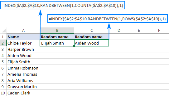
Supposing you have a list of names in cells A2:A10 and you want to randomly select one name from the list. This can be done by using one of the following formulas:
=INDEX($A$2:$A$10,RANDBETWEEN(1,COUNTA($A$2:$A$10)),1)
or
=INDEX($A$2:$A$10,RANDBETWEEN(1,ROWS($A$2:$A$10)),1)
That's it! Your random name picker for Excel is all set up and ready to serve:
Note. Please be aware that RANDBETWEEN is a volatile function, meaning it will recalculate with every change you make to the worksheet. As the result, your random selection will also change. To prevent this from happening, you can copy the extracted name and paste it as value to another cell (Paste Special > Values). For the detailed instructions, please see How to replace formulas with values.
Naturally, these formulas can not only pick random names, but also select random numbers, dates, or any other random cells.
How these formulas work
In a nutshell, you use the INDEX function to extract a value from the list based on a random row number returned by RANDBETWEEN.
More specifically, the RANDBETWEEN function generates a random integer between the two values you specify. For the lower value, you supply the number 1. For the upper value, you use either COUNTA or ROWS to get the total row count. As the result, RANDBETWEEN returns a random number between 1 and the total count of rows in your dataset. This number goes to the row_num argument of the INDEX function telling it which row to pick. For the column_num argument, we use 1 since we want to extract a value from the first column.
Note. This method works well for selecting one random cell from a list. If your sample is supposed to include several cells, the above formula may return several occurrences of the same value because the RANDBETWEEN function is not duplicate-free. It is especially the case when you are picking a relatively big sample from a relatively small list. The next example shows how to do random selection in Excel without duplicates.
How to randomly select in Excel without duplicates
There are a few ways to select random data without duplicates in Excel. Generally, you'd use the RAND function to assign a random number to each cell, and then you pick a few cells by using an Index Rank formula.
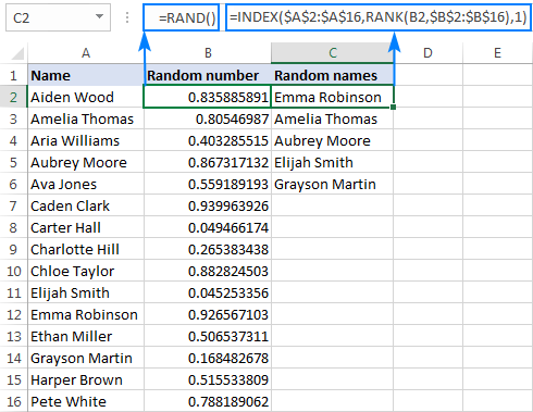
With the list of names in cells A2:A16, please follow these steps to extract a few random names:
- Enter the Rand formula in B2, and copy it down the column:
=RAND() - Put the below formula in C2 to extract a random value from column A:
=INDEX($A$2:$A$16, RANK(B2,$B$2:$B$16), 1) - Copy the above formula to as many cells as many random values you want to pick. In our case, we copy the formula to four more cells (C2:C6).
That's it! Five random names are extracted without duplicates:
How this formula works
Like in the previous example, you use the INDEX function to extract a value from column A based on a random row coordinate. In this case, it takes two different functions to get it:
- The RAND formula populates column B with random numbers.
- The RANK function returns the rank a random number in the same row. For example, RANK(B2,$B$2:$B$16) in cell C2 gets the rank of the number in B2. When copied to C3, the relative reference B2 changes to B3 and returns the rank of the number in B3, and so on.
- The number returned by RANK is fed to the row_num argument of the INDEX function, so it picks the value from that row. In the column_num argument, you supply 1 because you want to extract a value from the first column.
A word of caution! As shown in the screenshot above, our Excel random selection contains only unique values. But theoretically, there is a slim chance of duplicates appearing in your sample. Here's why: on a very large dataset, RAND might generate duplicate random numbers, and RANK will return the same rank for those numbers. Personally, I've never got any duplicates during my tests, but in theory, such probability does exist.
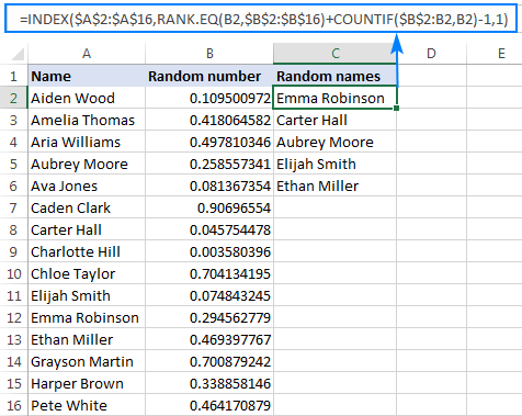
If you are looking for a bulletproof formula to get a random selection with only unique values, then use RANK + COUNTIF or RANK.EQ + COUNTIF combination instead of just RANK. For the detailed explanation for the logic, please see Unique ranking in Excel.
The complete formula is a bit cumbersome, but 100% duplicate-free:
=INDEX($A$2:$A$16, RANK.EQ(B2, $B$2:$B$16) + COUNTIF($B$2:B2, B2) - 1, 1)
Notes:
- Like RANDBETWEEN, the Excel RAND function also generates new random numbers with each recalculation of your worksheet, causing the random selection to change. To keep your sample unchanged, copy it and paste somewhere else as values (Paste Special > Values).
- If the same name (number, date, or any other value) appears more than once in your original data set, a random sample might also contain several occurrences of the same value.
More ways to get a random selection with no repeats in Excel 365 - 2010 are described here: How to get random sample in Excel without duplicates.
How to select random rows in Excel
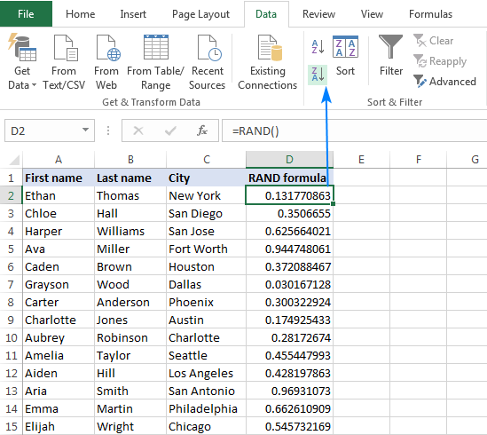
In case your worksheet contains more than one column of data, you can select a random sample in this way: assign a random number to each row, sort those numbers, and select the required number of rows. The detailed steps follow below.
- Insert a new column to the right or to the left of your table (column D in this example).
- In the first cell of the inserted column, excluding the column headers, enter the RAND formula:
=RAND() - Double-click the fill handle to copy the formula down the column. As the result, you will have a random number assigned to each row.
- Sort the random numbers largest to smallest (sorting in ascending order would move the column headers at the bottom of the table, so be sure to sort descending). For this, head over to the Data tab > Sort & Filter group, and click the ZA button. Excel will automatically expand the selection and sort the entire rows in random order.
If you are not quite satisfied with how your table has been randomized, hit the sort button again to resort it. For the detailed instructions, please see How to randomly sort in Excel.
- Finally, select the required number of rows for your sample, copy them and paste to wherever you like.
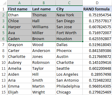
To have a closer look at the formulas discussed in this tutorial, you are welcome to download our sample workbook to Excel Random Selection.
How to randomly select in Excel with Randomize tool
Now that you know a handful of formulas to get a random sample in Excel, let's see how you can achieve the same result in a mouse click.
With Random Generator for Excel included in our Ultimate Suite, here's what you do:
- Select any cell in your table.
- Go to the Ablebits Tools tab > Utilities group, and click Randomize > Select Randomly:
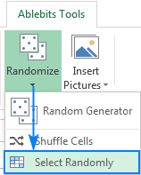
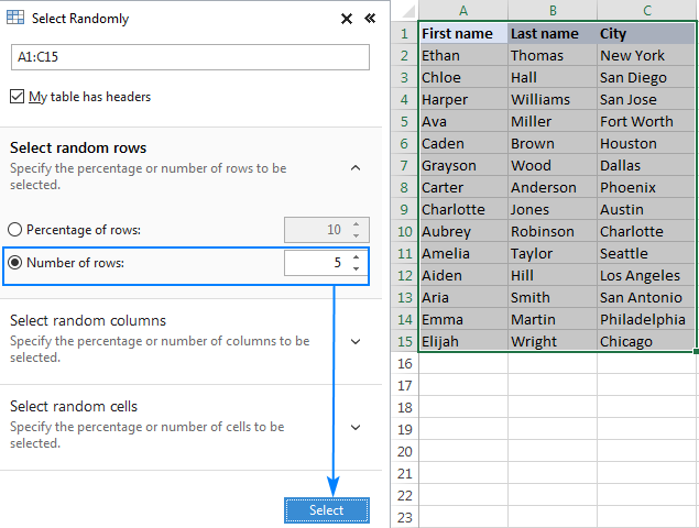
- On the add-in's pane, choose what to select: random rows, random columns or random cells.
- Specify the number or percentage for the desired sample size.
- Click the Select button. Done!
For example, this is how we can select 5 random rows from our sample data set:
And you will get a random selection in a second:
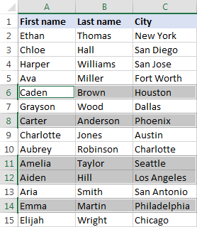
Now, you can press Ctrl + C to copy your random sample, and then press Ctrl + V to paste it to location in the same or another sheet.
If you'd like to test the Randomize tool in your worksheets, just grab a trial version of Ultimate Suite below. In case your are using Google spreadsheets, you may find our Random Generator for Google Sheets useful.
Available downloads
Selecting random sample - formula examples (.xlsx file)
Ultimate Suite - trial version (.exe file)
 by
by
50 comments
I have used the following formula, which gives me an error.
I am trying to pull random from another worksheet named Key.
=INDEX(Key!$B$28:$B$69,RANK($C$28:$C$69),1)
Also If I am able to make this work& I need it to pull randomly month without repeating, is there something I should add to this? Is there a way to make it start over when all selections have been randomly selected?
Thank you for your help.
Hi! Please take a look at this article: How to get random sample in Excel without duplicates. I hope it’ll be helpful.
how to record the output of generated random number
The fastest way is to replace formulas with calculated values. You will find step-by-step instructions in the above linked tutorial.
Hi! How are you am looking for a formular that will pick numbers rondomly in any cell in each row in each column and sum the picked number to give a given set sum. E.g.
A. B. C
2.34. 2.45. 2.56
2.56. 2.78. 2.58
2.45. 2.76. 3.89
I am looking for the formular that will randomly pick the data above which will give me this total 9.01 though this total may differ according to my needs
Hi!
Add to the INDEX formula you see in this article a random column selection.
=INDEX(A2:C15,RANDBETWEEN(1,COUNTA($A$2:$A$15)), RANDBETWEEN(1,COUNTA($A$2:$C$2)))
You can learn more about INDEX in this article: Excel INDEX function with formula examples.
Hello,
I have a list of about 12,000 clients and would like to do a study on a few of them without biased selection. How do I get the random sample and determine the best sample size in Excel. if the selected random numbers would be 'highlighted'. I have tried using RAND() but not helping out as I would like. thanks so much for the help.
Hello!
You did not mention what problem you have with the RAND function.
But, we have a ready-made solution for your task.
I'd recommend you to have a look at our Ablebits Tools - Randomize.
It is available as a part of our Ultimate Suite for Excel that you can install in a trial mode and check how it works for free.
Hi, Thanks for the reply.
RAND keeps recalculating that by the time I paste values, the figures have already changed. am not able to know what percentile to take to avoid bias or have minimal error. I would a function that would help say for 500 clients you can sample out maybe 149, one with 1000 one can sample 253. like define a range for me and thereafter be able to Vlookup those particular IDs. thanks again
Hello,
I see that the sorted list of random numbers in your screenshot for the option of how to select random rows in a spreadsheet is running into the same problem as I am: numbers are not sorting correctly. I don't understand how Excel is sorting the numbers. Can you help?
Stefan
Hello!
Please note that after sorting, you see completely different numbers. Excel sorts the old numbers first. The RAND function then immediately generates new ones instead. This example uses sorting to cause the RAND function to generate new random numbers.
If you need a correct sort, replace the formulas in the cells with numbers using Paste Special.
Hey!
Thanks for the great info.
If I want the selection to be done only is part of the list, how can I modify the formula to specify the different group of cells to look at? (when I just add the different groups, I get a VALOR error)
Thanks!
Hello!
Please describe your problem in more detail. What formula did you want to change? What result did you want to get? It’ll help me understand it better and find a solution for you. Thank you.
I have my data organised into rows and want to select one cell randomly from each row. Is there a straightforward way of doing this?
Same problem for me
Hi! To extract from a range of values use the INDEX function .
Suppose you have a range in cells A1:D10, and you want to randomly select one value of each row. Insert a new column to the right of your table (let’s say column E). In the first cell of the inserted column, enter the formula:
=INDEX($A$1:$D$10, ROW(A1), RANDBETWEEN(1, COUNTA(A1:D1)))
The ROW function returns the row number in the range. The RANDBETWEEN function randomly selects the column number.
Double-click the fill handle to copy the formula down the column. Each row will now have a random number assigned to it.
Hi, what if I want to get only 5 random non-duplicate names from A column?
Hi Garry,
Just want to let you know that we have published a new tutorial that describes a few easy solutions to randomly select in Excel without duplicates, including the use of the new Excel dynamic array functions: How to get random sample in Excel without duplicates
Hello Garry!
If I understand your task correctly, read carefully the section above Random selection without duplicates. If after that there will be specific questions - ask.
Hi
could you help me with the formula for the below data
In sheet one, I have some data (example below)
1 - Apple
1 - Orange
2 - banana
2 - Peach
If 1 is input, then a random value from 1 (Apple or Orange) Should be returned. If 2 is input, then a value from 2 list (either banana or peach ) should be returned. If 3 is input, it should return a error.
Hello!
If I understand your task correctly, the following formula should work for you:
=IF(F2=1,INDEX($B$1:$B$2,RANDBETWEEN(1,COUNTA($B$1:$B$2)),1), IF(F2=2,INDEX($B$3:$B$4,RANDBETWEEN(1,COUNTA($B$3:$B$4)),1),"ERROR"))
Hi, thank you for your help.
In case of dynamic values, what should I do i.e the number of values under 1 will keep increasing, say now I have Apple and orange. tomorrow it might be Apple, Orange and Grapes under 1. SO if a match of 1 is found, then it should return a random value(Apple/Orange/grapes). Please help.
Hello!
If I understand your task correctly, the following formula should work for you:
=IF(F3 < 3,INDEX($B$2:$B$21,SMALL(IF($A$2:$A$21=$F$3,ROW($A$2:$A$21)-1,""), ROUNDUP(COUNTIF($A$2:$A$21,$F$3)*RAND(),0))),"ERROR")
The formula selects values from column B for which, by condition, 1 or 2 is written in column A. One of these values is randomly displayed.
The condition is written in cell F3
I hope this will help
This is the formula I'm using to get a random selection
=INDEX($B$2:$B194,RANDBETWEEN(1,COUNTA($B$2:$B$194)),1)
Hello Janet!
Thank you for your reply.
To stop automatic workbook calculation, please try one more method. Please go to File – Options – Formulas – Calculation Options, choose the Manual option and uncheck the box next to "Recalculate workbook before saving". After you do this, the formulas will be recalculated by clicking F9.
To choose random values, you may try to use the following formula:
=INDEX( IFERROR( INDEX($B$2:$B$194, SMALL(IF($C$2:$C$194<>1, ROW(INDIRECT("1:"&ROWS($C$2:$C$194)))), ROW(INDIRECT("1:"&ROWS($C$2:$C$194))))),""), RANDBETWEEN(1,COUNTIF($C$2:$C$194,"<>1")),1)
Suppose, you mark the values that have already been used with number “1” in column C, so they won’t be selected again.
I hope these recommendations will be helpful for you.
Is there a way to stop it from changing the random selection every time anything is edited in the workbook? The formulas work great and I am able to get my random sample, but every time any cell is changed the selection changes. I just want it to generate a list and not change once I have the list. Thanks!
Glad I read comments, I have the exact same question.
Hello Janet! Hello Tim!
If you are using the formula for random selection and can't make the result stay unchanged, there are three possible solutions:
1 - Replace the formulas with values. Just copy the cell(s) with your randomly generated values (CTRL+C), then use Paste Special (CTRL+ALT+V) to insert values.
2 - Disable the automatic calculation in your Excel. Go to File -> Options -> Formulas -> Calculation Options and switch from Automatic to Manual option there.
Note! In this case, you'll need to hit Shift+F9 to recalculate the formulas in any workbook you're working with.
3 - Disable the automatic calculation for the particular sheet. Just press ALT+F11, look through the properties of the sheet you're working with, find EnableCalculation parameter there and set False for it. Thus, all the worksheets will be recalculated automatically while the one you applied these changes for will be updated only when you use the Shift+F9 shortcut.
I hope this will help you. If however, this is not exactly what you meant, please specify and I'll try to find the right solution for you. Thank you.
Thank you! That stopped it from re-selecting each time I work in another cell, but for some reason, the SHIFT+F9 does not work to make a selection. It now returns a "0". The cells I'm trying to select from contain text only. I have a list of local businesses, and I need to choose one each week, till I have gone through all of them. I don't want to choose one twice, before I have chosen all of them. I set one column to place a check mark by once they are chosen, but it recalculates every time I put in my checkmark, and move out of that cell. Also, hopefully I will be adding businesses to my list, in the future. I don't want it to recalculate every time I add one.
Hello Svetlana Cheusheva
I can simply say that i fell in love with your work because i was looking for improve my skills and i found your explanation while searching in google and you provided it some working file too pretty impressive for learns like me and i still found lots of your articles and am definitely go through them you are good at sharing your knowledge thanks for doing that.
Have a wonderful day .
Thank you very much for your feedback, Srinivas! I am glad to hear you've found our tutorials helpful.
Ok...this may come across as a really silly question. The Randomizer picked the % of names I wanted, but now when I try to copy/paste, it's pasting the entire column, not just the selected names. What am I missing here?
Hi Amy,
Right after selecting the desired percentage of names, press Ctrl + C. This should copy only the selected cells.
hi Svetlana,
i would like to ask you that how to select entire column from a huge data sheet . ANY quick or short key for it. kindly reply to this message .
Hi Jeeson,
To select an entire column, simply click on its letter.
To select only the cells with data in a column, click on the topmost cell and press Ctrl + Shift + down arrow.
Hi,
I am trying to generate random names from a list using random numbers for 5 teams.
when I am trying to generate, there was repetition of same names in all the teams.
how to remove these repetition ?
Thanks
Hi Venkat,
If by coincidence some of the team members have identical names and you want to avoid any misunderstanding, it may be a good idea to put an index number into each cell where a player’s name is typed. It can easily be done with the help of an extra column containing numbers (from 1 to 10 if we are discussing a team of ten, for example) and the Ablebits ‘Merge Columns into One’ tool. Then I would advise you to opt for ‘Random Generator’ from the Ablebits ‘Randomize’ drop-down menu and make a ‘Custom list’ consisting of names accompanied by index numbers. Please note that the tool needs some empty cells reserved by you to complete the process. There won’t be any duplicates in the selection results if you click a small empty box next to ‘Unique values’ in the ‘Custom list’ menu marking it with a tick.
Hi,
I'm trying to create a randomly generated participant list from the database. I would like to select the few names based on the cities and gender. Do you have any idea how i would do that?
Thanks
Hi,
The selection process may be based on applying Ablebits’ ‘Random Generator’ and filtering. If you are working with a properly organized Excel table which has built-in filters, let them do that part of your task for you. If not, you can use Ablebits’ ‘Filter’ instead.
Hello,
I'm trying to create a randomly generated shopping list from a list of ingredients and the only limiting factor is the overall cost. Do you have any idea how i would do that?
Yes Nikko, I have made an excel sheet with macros built, where you have the limiting factor of samples for starting and ending numbers,
This will not work. I am trying to pick a word from a list. This formula just comes up with NAME?
Hi Julie,
To make things easier, you can download our sample workbook with all the formulas discussed in this tutorial and try them on your list.
Hi, Julie,
the NAME error usually means that you accidentally misspelled the name of the function.
Please make sure that everything in your formula is spelled correctly. If it is, please let me know what formula you used.
I'll try to help.
here's how i did on getting random without duplicates:
on b2 type your population or numbers 1,2,3,4,5,etc
on A1 type =rand() drag crosshair down to the number of selection next to b2 down.
on c1 type formula: =LARGE($A$1:$A$9,ROW(A1)) doubleclick crosshair
on D1 type =VLOOKUP(C1,$A$1:$B$9,2,0) doubleclick croshair
press delete on any blank cell to generate new random group
b2 column is your numbers you want ei. bingo numbers 1,2,3,...15
you assign random to each number =rand() on A1 downward for each number
on c1 column type formula to get the largest random number using formula =LARGE($A$1:$A$15,ROW(A1)) and double click crosshair to copy downward
vlookup top five numbers
press delete to generate new top five numbers
Hi,
Used your formula with the rank.eq and count if. It doesn't work on a large data set. Instead of picking random numbers it takes the first x amount of numbers and puts them in a random order.
Hi,
I have not tried the RANK.EQ + COUNTIF() although I had suspected it might not work because of the set up. However, if you multiply two RAND() functions, you get less likelihood of duplication in a large list.