The tutorial will teach you the most effective formulas to average numbers, percentages and times in Excel and avoid errors.
In Microsoft Excel, there exist a handful of different formulas for calculating average. This tutorial focuses on the most popular one - the AVERAGE function.
AVERAGE function in Excel
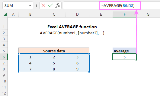
The AVERAGE function in Excel is used to find the arithmetic mean of specified numbers. The syntax is as follows:
Where number1, number2, etc. are numeric values for which you want to get the average. They can be supplied in the form of numeric values, arrays, cell or range references. The first argument is required, subsequent ones are optional. In one formula, you can include up to 255 arguments.
AVERAGE is available in all versions of Excel 365 though Excel 2007.
AVERAGE function - 6 things to know about
For the most part, using the AVERAGE function in Excel is easy. However, there are a few nuances that you should be aware of.
- Cells with zero values are included in the average.
- Empty cells are ignored.
- Cells containing text strings and logical values TRUE and FALSE are ignored. If you want to include Boolean values and text representations of numbers in the calculation, use the AVERAGEA function.
- Boolean values typed directly in a formula are counted. For example, the formula AVERAGE(TRUE, FALSE) returns 0.5, which is the average of 1 and 0.
- If the specified arguments do not contain a single valid numeric value, a #DIV/0! error occurs.
- Arguments that are error values cause an AVERAGE formula to return an error. To avoid this, please see how to average ignoring errors.
Note. When using the AVERAGE function in your Excel sheets, please do keep in mind the difference between cells with zero values and blank cells - 0's are counted, but empty cells are not. This might be especially confusing if the "Show a zero in cells that have a zero value" option is unchecked in a given worksheet. You can find this option under Excel Options > Advanced > Display options for this worksheet.
Excel AVERAGE formula
To build a basic Excel formula for average, all you need to do is to supply the source values. This can be done in a few different ways.
To calculate an average of certain numbers, you can type them directly in a formula. For example, to average the numbers 1,2,3, and 4, the formula is:
=AVERAGE(1,2,3,4)
To average a column in Excel, supply a whole-column reference:
=AVERAGE(A:A)
To average a row, use a whole-row reference:
=AVERAGE(1:1)
To average a range of cells, specify that range in your formula:
=AVERAGE(A1:C20)
To return a mean of non-adjacent cells, each cell reference should be supplied individually:
=AVERAGE(A1, C1, D1)
To average multiple ranges, use several range references in a single formula:
=AVERAGE(A1:A20, C1:D10)
And naturally, nothing prevents you from including values, cell and range references in the same formula as your business logic requires. For example:
=AVERAGE(B3:B5, D7:D9, E11, 100)
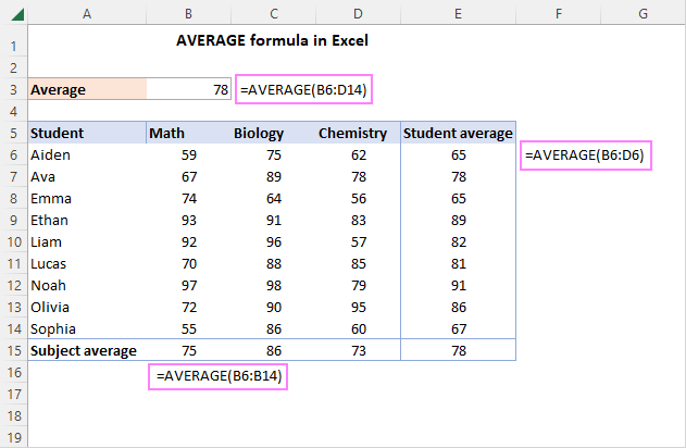
And here is a real-life scenario. In the below dataset, we use 3 different formulas for calculating an average - in the entire range, in each row and in each column:
How to use AVERAGE function in Excel - examples
Apart from numbers, Excel AVERAGE can easily find an arithmetic mean of other numeric values such as percentages and times, as demonstrated in the following examples.
Calculate average percentage in Excel
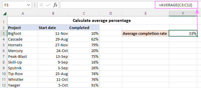
To get an average of percentages, you use a normal Excel formula for average. The key thing is to set the Percent format for the formula cell.
For example, to calculate an average percentage in cells C2 through C11, the formula is:
=AVERAGE(C2:C11)
Get average time in Excel
Calculating different time units manually, would be a real pain… Luckily, the Excel AVERAGE function copes with times perfectly. For the time average to display correctly, just remember to apply an appropriate time format to the formula cell.
For instance, to find an average time in the below dataset, the formula is:
=AVERAGE(B3:B13)

Excel average without zeros
The Excel AVERAGE function skips blank cells, text and logical values, but not zeros. In the image below, notice that the average in cells E4, E5 and E6 is the same as in E3 as a blank cell and invalid values in column C are ignored and only the numbers in columns B and D are processed. However, the zero value in C7 is included in the average in E7, since it is a valid numeric value.

To exclude zeros, use the AVERAGEIF or AVERAGEIFS function instead. For example:
=AVERAGEIF(B3:D3, "<>0")

Average top or bottom N values
To get an average of top 3, 5, 10 or n values in a range, use AVERAGE in combination with the LARGE function:
For instance, to get an average of the 3 largest numbers in B3:B11, the formula is:
=AVERAGE(LARGE(B3:B11, {1,2,3}))
To calculate a mean of bottom 3, 5, 10 or n values in a range, use AVERAGE together with the SMALL function:
For instance, to average the 3 lowest numbers in the range, the formula goes as follows:
=AVERAGE(SMALL (B3:B11, {1,2,3}))
And here are the results:

How this formula works:
Normally, the LARGE function determines the Nth largest value in a given array. To get the top n values, an array constant such as {1,2,3} is used for the second argument.
In our case, LARGE returns the highest 3 values in the range, which are 94, 93 and 90. AVERAGE takes it from there and outputs the mean.
The AVERAGE SMALL combination works in a similar way.
AVERAGE IF formula in Excel
To calculate an average with conditions, you can leverage AVERAGEIF or AVERAGEIFS in Excel 2007 - 365. In earlier versions, you can construct your own AVERAGE IF formula.
AVERAGE IF with one condition
To average numbers that meet a certain condition, use this generic formula:
In Excel 2019 and lower, this only works as an array formula, meaning you need to press the Ctrl + Shift + Enter keys to complete it correctly. In Excel 365 and 2021, a normal formula will work nicely.
As an example, let's find an average Math score in the table below. For this, just use "Math" for criteria:
=AVERAGE(IF(C3:C11="Math", B3:B11))
Or you can input the condition in some cell and reference that cell (F2 in our case):
=AVERAGE(IF(C3:C11=F2, B3:B11))))

How this formula works
The logical test of the IF function compares each subject in C3:C11 against the target one in F2. The result of the comparison is an array of TRUE and FALSE values, where TRUEs represent matches:
{FALSE;FALSE;FALSE;TRUE;TRUE;FALSE;FALSE;TRUE;FALSE}
For the value_ if_true argument, we supply the range of scores (B3:B11), so if the logical test is TRUE, the corresponding score is returned. As the value_ if_false argument is omitted, FALSE appears where the condition is not met:
{FALSE;FALSE;FALSE;74;67;FALSE;FALSE;59;FALSE}
This array is fed to the AVERAGE function, which calculates an arithmetic mean of the numbers ignoring the FALSE values.
AVERAGE IF with multiple criteria
To average numbers with several criteria, the generic formula is:
For example, to average the Math scores in class A, you can use this formula:
=AVERAGE(IF((C3:C11="Math") * (D3:D11="A"), B3:B11))
With cell references for criteria, this works equally well:
=AVERAGE(IF((C3:C11=G2) * (D3:D11=G3), B3:B11))
In Excel 2019 and lower, both of the above should be array formulas, so remember to press Ctrl + Shift + Enter to get an accurate result. In Excel 365 and 2021, a normal Enter key will work fine due to inbuilt support for dynamic arrays.
The same result can be achieved with the help of the nested IF statement:
=AVERAGE(IF(C3:C11=G2, IF(D3:D11=G3, B3:B11)))
Which formula to use is just a matter of your personal preference.

How this formula works
In the logical test of IF, two comparison operations are performed - first, you check the list of subjects in C3:C11 against the value in G2, and then you compare the classes in D3:D11 against the value in G3. The two arrays of TRUE and FALSE values are multiplied, and the multiplication operation works like the AND operator. In any arithmetic operation, TRUE equates to 1 and FALSE equates to 0. Multiplying by 0 always gives zero, so the resulting array has 1 only when both conditions are TRUE. This array is evaluated in the logical test of the IF function, which returns the scores corresponding to 1's (TRUE):
{FALSE;FALSE;FALSE;74;67;FALSE;FALSE;FALSE;FALSE}
This final array is served to AVERAGE.
How to round an average in Excel
In case you wish to round only the displayed average without changing the underlying value, make use of the Decrease Decimal command on the ribbon or the Format Cells dialog box as explained in How to round average in Excel.
To round the calculated value itself, combine AVERAGE with one of the Excel rounding functions.
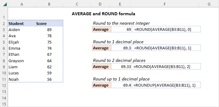
To follow the general math rules for rounding, nest AVERAGE in the ROUND function. In the 2nd argument (num_digits), specify the number of digits to round an average to.
For example, to round an average to the nearest integer, use this formula:
=ROUND(AVERAGE(B3:B11), 0)
To round an average to one decimal place, use 1 for the num_digits argument:
=ROUND(AVERAGE(B3:B11), 1)
To round an average to two decimal places, use 2 for the num_digits argument:
=ROUND(AVERAGE(B3:B11), 2)
And so on.
For rounding upward, use the ROUNDUP function:
=ROUNDUP(AVERAGE(B3:B11), 1)
For rounding downward, ROUNDDOWN is the function to use:
=ROUNDDOWN(AVERAGE(B3:B11), 1)
Fixing #DIV/0 error in Excel AVERAGE
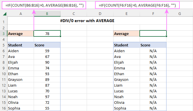
If the range of cells you are trying to calculate has no numeric values, an AVERAGE formula will return a divide by zero error (#DIV/0!). To fix this, you can get a total of numeric values with the COUNT function and if the count is greater than 0, then average; otherwise - return an empty string.
For example, to avoid a #DIV/0 error with average in the below data set, use this formula:
=IF(COUNT(B6:B16)>0, AVERAGE(B6:B16), "")
Average and ignore errors
When attempting to average a range of cells that has any errors, the result will be an error. To prevent this from happening, use one of the following solutions.
AVERAGE and IFERROR
Before averaging, filter out errors with the help of the IFERROR function:
In all versions except Excel 365 and 2021 where arrays are handled natively, hit the Ctrl + Shift + Enter keys together to make it an array formula.
For example, to average the below range of cells without errors, the formula is:
=AVERAGE(IFERROR(B3:B13, ""))
AGGREGATE function
Another easy way to average ignoring errors is using the AGGREGATE function. To configure AGGREGATE for this purpose, you set the function_num argument to 1 (AVERAGE function), and the options argument to 6 (ignore error values).
For instance:
=AGGREGATE(1, 6, B3:B13)
As you can see in the screenshot, both functions work beautifully:

Excel AVERAGE not working
If you've faced a problem with an AVERAGE formula in Excel, our troubleshooting tips will help you quickly resolve it.
Numbers formatted as text
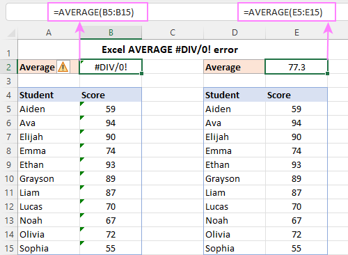
If the range you are attempting to average does not have a single numeric value, a #DIV/0 error occurs. This often happens when numbers are formatted as text. To fix the error, simply convert text to number.
A small green triangle in the top-left corner of the cells is a clear indication of this case:
Error values in the referred cells
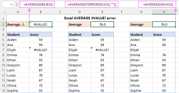
If an AVERAGE formula refers to cells that contain some error, say #VALUE!, the formulas will result in the same error. To solve this problem, use a combination of AVERAGE along with IFERROR or the AGGREGATE function as described in these examples. Or replace the value error in the source data with some text if applicable.
AVERAGE formula shows up in a cell instead of the result
If your cell displays a formula instead of the answer, then most likely the Show Formulas mode is on in your worksheet. Other reasons could be a formula entered as text, with a leading space or apostrophe before the equal sign. The solutions to all these problems are provided here: Excel formulas not calculating.
That's how you use the AVERAGE function in Excel to find an arithmetic mean. I thank you for reading and hope to see you on our blog next week!
Practice workbook for download
AVERAGE formula in Excel - examples (.xlsx file)
 by
by
10 comments
I want to calculate the average of a row, say row 11, that has 22 columns (D thru X), I only want to average the last 10 entries, it should ignore blanks and exclude the maximum and minimum values within those last 10 entries.
Hello Mike!
You want an average of the last 10 filled cells in row 11 (columns D:X), ignoring blanks, and then excluding the maximum and minimum among those 10.
Since your data is in row 11 from D11:X11, we will extract the last 10 non-blank numbers. One way is with the TAKE function + FILTER function (Excel 365)
=TAKE(FILTER(D11:X11,ISNUMBER(D11:X11)), -10)
Exclude the max and min, then average the rest. Wrap it with AVERAGE, MAX function, and MIN finction.
Here is how you can do it in Excel with a formula:
= (SUM(TAKE(FILTER(D11:X11,ISNUMBER(D11:X11)),,-10)) - MAX(TAKE(FILTER(D11:X11,ISNUMBER(D11:X11)),,-10)) - MIN(TAKE(FILTER(D11:X11,ISNUMBER(D11:X11)),,-10))) / 8
Hi, I am trying to create a formula that will create a running average, starting in cell I2, with a value being added to each subsequent cell below. At this point I am at cell I92, and tomorrow I will be populating cell I93, and so on. For the range I2:I92, I want the average to appear in J92. And for the range I2:I93, I want the average to appear in J93, and so on.
Any help would be greatly appreciated.
Thanks,
Bob
Hi Bob,
We have a separate tutorial on running average, please check it out: Excel moving average (running average) formula.
I have 10 employees and need calculate their average percentage weekly, monthly and quarterly.
For Example:
Joe Cell C1, Sam Cell D1, Greg Cell E1
1st week
2nd week
3rd week
4th week
Joe will be =average(C2:C5)
How do I create a formula for Sam (D2:D5) and Greg (E2:E5) and multiply employees without having to manually enter for each cell. This we’ll be for the entire year, 52 weeks for each employee. I tried everything to copy paste formula, drag cell, etc but gives me that same results if be consecutive of only Cell C2:C5, C6:C9, etc. any help will be great. I have been researching testing and nothing is working. TIA
Hello! To calculate the average value for each 4 weeks, you can use the OFFSET function. Write this formula, for example, in cell K2 and copy down the column:
=AVERAGE(OFFSET($С$2,(ROW(A1)-1)*4,0,4,1))
My =Average() formula results in a date. How to fix it?
Hi! Change the format of the cell with the formula to General.
What if I need the average of three cells that are not a range, but need to not count the zeros? For example:
=AVERAGE('Carrier #1'!C3,'Carrier #1'!AS4,'Carrier #1'!CI4)
Hi! Unfortunately, the method suggested in the article Excel average without zeros cannot be used for you, because the AVERAGEIFS function only works with cell ranges, not individual cells. Here's a sample formula for you:
=SUM(A1+A2+A3)/((A1>0)+(A2>0)+(A3>0))