Comparing columns in Excel is something that we all do once in a while. Microsoft Excel offers a number of options to compare and match data, but most of them focus on searching in one column. In this tutorial, we will explore several techniques to compare two columns in Excel and find matches and differences between them.
How to compare 2 columns in Excel row-by-row
When you do data analysis in Excel, one of the most frequent tasks is comparing data in each individual row. This task can be done by using the IF function, as demonstrated in the following examples.
Example 1. Compare two columns for matches or differences in the same row
To compare two columns in Excel row-by-row, write a usual IF formula that compares the first two cells. Enter the formula in some other column in the same row, and then copy it down to other cells by dragging the fill handle (a small square in the bottom-right corner of the selected cell). As you do this, the cursor changes to the plus sign:
To find cells within the same row having the same content, A2 and B2 in this example, the formula is as follows: To find cells in the same row with different values, simply replace the equals sign with the non-equality sign (<>): And of course, nothing prevents you from finding both matches and differences with a single formula: Or The result may look similar to this:
As you see, the formula handles numbers, dates, times and text strings equally well. Tip. You can also compare two columns row-by-row using Excel Advanced Filter. Here is an example showing how to filter matches and differences between 2 columns.
Formula for matches
=IF(A2=B2,"Match","")
Formula for differences
=IF(A2<>B2,"No match","")
Matches and differences
=IF(A2=B2,"Match","No match")=IF(A2<>B2,"No match","Match")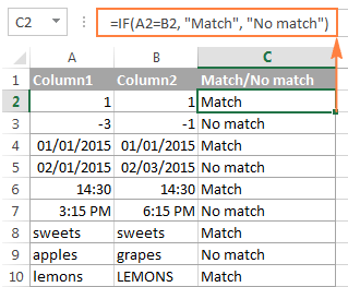
Example 2. Compare two lists for case-sensitive matches in the same row
As you have probably noticed, the formulas from the previous example ignore case when comparing text values, as in row 10 in the screenshot above. If you want to find case-sensitive matches between 2 columns in each row, then use the EXACT function:
=IF(EXACT(A2, B2), "Match", "")
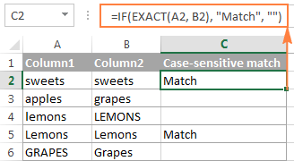
To find case-sensitive differences in the same row, enter the corresponding text ("Unique" in this example) in the 3rd argument of the IF function, e.g.:
=IF(EXACT(A2, B2), "Match", "Unique")
Compare multiple columns for matches in the same row
In your Excel worksheets, multiple columns can be compared based on the following criteria:
- Find rows with the same values in all columns (Example 1)
- Find rows with the same values in any 2 columns (Example 2)
Example 1. Find matches in all cells within the same row
If your table has three or more columns and you want to find rows that have the same values in all cells, an IF formula with an AND statement will work a treat:
=IF(AND(A2=B2, A2=C2), "Full match", "")
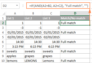
If your table has a lot of columns, a more elegant solution would be using the COUNTIF function:
=IF(COUNTIF($A2:$E2, $A2)=5, "Full match", "")
Where 5 is the number of columns you are comparing.
Example 2. Find matches in any two cells in the same row
If you are looking for a way to compare columns for any two or more cells with the same values within the same row, use an IF formula with an OR statement:
=IF(OR(A2=B2, B2=C2, A2=C2), "Match", "")
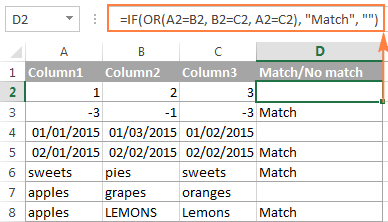
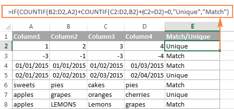
In case there are many columns to compare, your OR statement may grow too big in size. In this case, a better solution would be adding up several COUNTIF functions. The first COUNTIF counts how many columns have the same value as in the 1st column, the second COUNTIF counts how many of the remaining columns are equal to the 2nd column, and so on. If the count is 0, the formula returns "Unique", "Match" otherwise. For example:
=IF(COUNTIF(B2:D2,A2)+COUNTIF(C2:D2,B2)+(C2=D2)=0,"Unique","Match")
How to compare two columns in Excel for matches and differences
Suppose you have 2 lists of data in Excel, and you want to find all values (numbers, dates or text strings) which are in column A but not in column B.
For this, you can embed the COUNTIF($B:$B, $A2)=0 function in IF's logical test and check if it returns zero (no match is found) or any other number (at least 1 match is found).
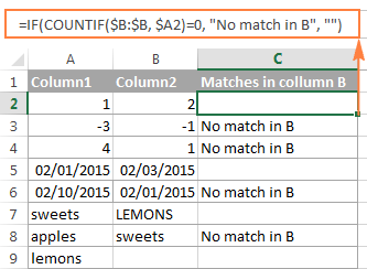
For instance, the following IF/COUNTIF formula searches across the entire column B for the value in cell A2. If no match is found, the formula returns "No match in B", an empty string otherwise:
=IF(COUNTIF($B:$B, $A2)=0, "No match in B", "")
Tip. If your table has a fixed number of rows, you can specify a certain range (e.g. $B2:$B10) rather than the entire column ($B:$B) for the formula to work faster on large data sets.
The same result can be achieved by using an IF formula with the embedded ISERROR and MATCH functions:
=IF(ISERROR(MATCH($A2,$B$2:$B$10,0)),"No match in B","")
Or, by using the following array formula (remember to press Ctrl + Shift + Enter to enter it correctly):
=IF(SUM(--($B$2:$B$10=$A2))=0, " No match in B", "")
If you want a single formula to identify both matches (duplicates) and differences (unique values), put some text for matches in the empty double quotes ("") in any of the above formulas. For example:
=IF(COUNTIF($B:$B, $A2)=0, "No match in B", "Match in B")
How to compare two lists in Excel and pull matches
Sometimes you may need not only match two columns in two different tables, but also pull matching entries from the lookup table. Microsoft Excel provides a special function for this - the VLOOKUP function. As an alternative, you can use a more powerful and versatile INDEX MATCH formula. The users of Excel 2021 and Excel 365, can accomplish the task with the XLOOKUP function.
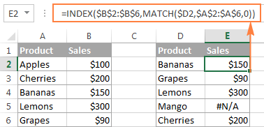
For example, the following formulas compare the product names in columns D against the names in column A and pull a corresponding sales figure from column B if a match is found, otherwise the #N/A error is returned.
=VLOOKUP(D2, $A$2:$B$6, 2, FALSE)
=INDEX($B$2:$B$6, MATCH($D2, $A$2:$A$6, 0))
=XLOOKUP(D2, $A$2:$A$6, $B$2:$B$6)
For more information, please see How to compare two columns using VLOOKUP.
If you don't feel very comfortable with formulas, you can have the job done using a fast and intuitive solution - Merge Tables Wizard.
Compare two lists and highlight matches and differences
When you compare columns in Excel, you may want to "visualize" the items that are present in one column but missing in the other. You can shade such cells in any color of your choosing by using the Excel Conditional Formatting feature and the following examples demonstrate the detailed steps.
Example 1. Highlight matches and differences in each row
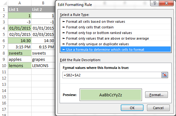
To compare two columns and Excel and highlight cells in column A that have identical entries in column B in the same row, do the following:
- Select the cells you want to highlight (you can select cells within one column or in several columns if you want to color entire rows).
- Click Conditional formatting > New Rule… > Use a formula to determine which cells to format.
- Create a rule with a simple formula like
=$B2=$A2(assuming that row 2 is the first row with data, not including the column header). Please double check that you use a relative row reference (without the $ sign) like in the formula above.
To highlight differences between column A and B, create a rule with this formula:
=$B2<>$A2
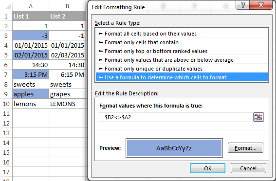
If you are new to Excel conditional formatting, please see How to create a formula-based conditional formatting rule for step-by-step instructions.
Example 2. Highlight unique entries in each list
Whenever you are comparing two lists in Excel, there are 3 item types that you can highlight:
- Items that are only in the 1st list (unique)
- Items that are only in the 2nd list (unique)
- Items that are in both lists (duplicates) - demonstrated in the next example.
This example demonstrates how to color the items that are only in one list.
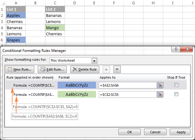
Supposing your List 1 is in column A (A2:A6) and List 2 in column C (C2:C5). You create the conditional formatting rules with the following formulas:
Highlight unique values in List 1 (column A):
=COUNTIF($C$2:$C$5, $A2)=0
Highlight unique values in List 2 (column C):
=COUNTIF($A$2:$A$6, $C2)=0
And get the following result:
Example 3. Highlight matches (duplicates) between 2 columns
If you closely followed the previous example, you won't have difficulties adjusting the COUNTIF formulas so that they find the matches rather than differences. All you have to do is to set the count greater than zero:
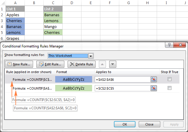
Highlight matches in List 1 (column A):
=COUNTIF($C$2:$C$5, $A2)>0
Highlight matches in List 2 (column C):
=COUNTIF($A$2:$A$6, $C2)>0
Highlight row differences and matches in multiple columns
When comparing values in several columns row-by-row, the quickest way to highlight matches is creating a conditional formatting rule, and the fastest way to shade differences is embracing the Go To Special feature, as demonstrated in the following examples.
Example 1. Compare multiple columns and highlight row matches
To highlight rows that have identical values in all columns, create a conditional formatting rule based on one of the following formulas:
=AND($A2=$B2, $A2=$C2)
or
=COUNTIF($A2:$C2, $A2)=3
Where A2, B2 and C2 are the top-most cells and 3 is the number of columns to compare.
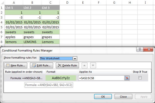
Of course, neither AND nor COUNTIF formula is limited to comparing only 3 columns, you can use similar formulas to highlight rows with the same values in 4, 5, 6 or more columns.
Example 2. Compare multiple columns and highlight row differences
To quickly highlight cells with different values in each individual row, you can use Excel's Go To Special feature.
- Select the range of cells you want to compare. In this example, I've selected cells A2 to C8.

By default, the top-most cell of the selected range is the active cell, and the cells from the other selected columns in the same row will be compared to that cell. As you can see in the screenshot above, the active cell is white while all other cells of the selected range are highlighted. In this example, the active cell is A2, so the comparison column is column A.
To change the comparison column, use either the Tab key to navigate through selected cells from left to right, or the Enter key to move from top to bottom.
Tip. To select non-adjacent columns, select the first column, press and hold Ctrl, and then select the other columns. The active cell will be in the last column (or in the last block of adjacent columns). To change the comparison column, use the Tab or Enter key as described above.
- On the Home tab, go to Editing group, and click Find & Select > Go To Special… Then select Row differences and click the OK button.
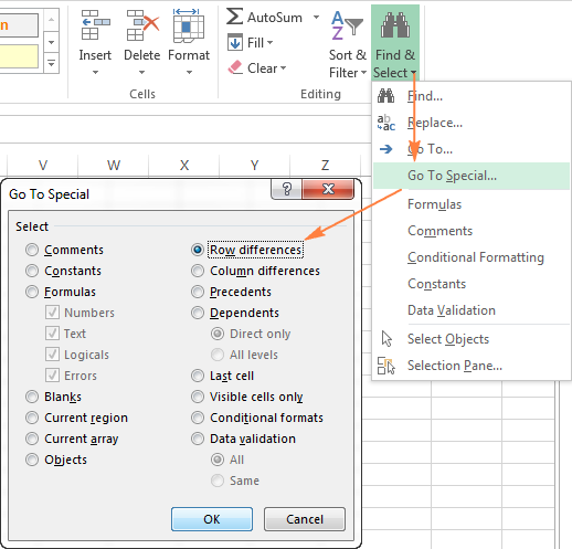
- The cells whose values are different from the comparison cell in each row are colored. If you want to shade the highlighted cells in some color, simply click the Fill Color icon on the ribbon and select the color of your choosing.

How to compare two cells in Excel
In fact, comparing 2 cells is a particular case of comparing two columns in Excel row-by-row except that you don't have to copy the formulas down to other cells in the column.
For example, to compare cells A1 and C1, you can use the following formulas.
For matches:
=IF(A1=C1, "Match", "")
For differences:
=IF(A1<>C1, "Difference", "")
To learn a few other ways to compare cells in Excel, please see:
Formula-free way to compare two columns / lists in Excel
Now that you know Excel's offerings for comparing and matching columns, let me show you our own solution for this task. This tool is named Compare Two Tables and it is included in our Ultimate Suite.
The add-in can compare two tables or lists by any number of columns and both identify matches/differences (as we did with formulas) and highlight them (as we did with conditional formatting).
For the purpose of this article, we'll be comparing the following 2 lists to find common values that are present in both.

To compare two lists, here are the steps you need to follow:
- Start with clicking the Compare Tables button on the Ablebits Data tab.

- Select the first column/list and click Next. In terms of the add-in, this is your Table 1.

- Select the second column/list and click Next. In terms of the add-in, it is your Table 2, and it can reside in the same or different worksheet or even in another workbook.

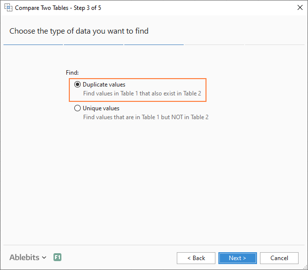
- Choose what kind of data to look for:
- Duplicate values (matches) - the items that exist in both lists.
- Unique values (differences) - the items that are present in list 1, but not in list 2.
Since our aim is to find matches, we select the first option and click Next.
- This is the key step where you select the columns for comparison. In our case, the choice is obvious as we are only comparing 2 columns: 2000 Winners against 2021 Winners. In bigger tables, you can select several column pairs to compare by.

- In the final step, you choose how to deal with the found items and click Finish.
A few different options are available here. For our purposes, these two are most useful:
- Highlight with color - shades matches or differences in the selected color (like Excel conditional formatting does).
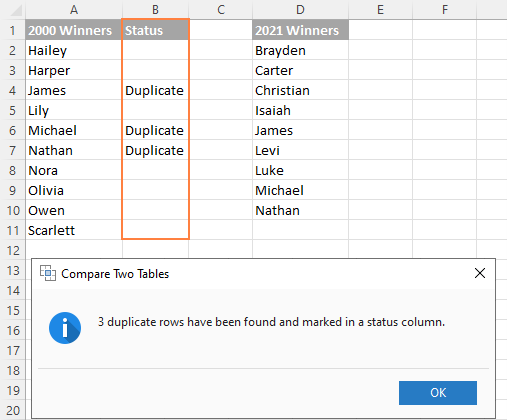
- Identify in the Status column - inserts the Status column with the "Duplicate" or "Unique" labels (like IF formulas do).
For this example, I've decided to highlight duplicates in the following color:
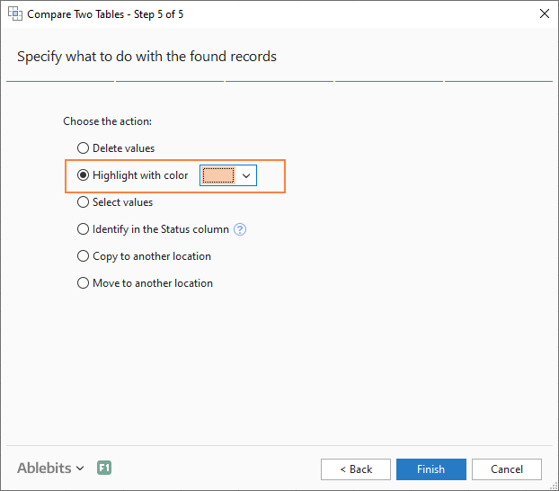
And in a moment, got the following result:

With the Status column, the result would look as follows:
Tip. If the lists you are comparing are in different worksheets or workbooks, it might be helpful to view Excel sheets side by side.
This is how you compare columns in Excel for matches (duplicates) and differences (unique values). If you are interested to try this tool, you are welcome to download an evaluation version using the below link.
I thank you for reading and encourage you to check out other helpful tutorials that we have :)
Available downloads
Compare Excel Lists - examples (.xlsx file)
Ultimate Suite - trial version (.exe file)
 by
by
548 comments
In first cell I have values like A,B,C and in 2nd cell I have value of B,A,C in this case both cell values are same but sequence is not match I want return value as True and if any value missed then false how to do it in excel
Hi!
Excel cannot compare text strings with different word orders. Split each text string into cells using a comma as a separator. You can read more about this here: Split string by delimiter or pattern, separate text and numbers or TEXTSPLIT function in Excel: split text strings by delimiter. Then compare the values using the IF function with AND and OR statements.
Thank you very much Alexander Trifuntov. Was looking for this for almost 4 hours.
Thank you once again for sharing the Template.
God Bless.
Thank you for your explanation but is there a function to know if two cells are on the same row in an other sheet ?
Hello!
I am not sure I fully understand what you mean. You can get the row number using the ROW function or CELL function
Good evening,
I have a unique 'multi-condition' question I'm using for scaled criteria in Excel.
I am matching paygrades (determined by O2, O3, O4, etc)
--but I am scaling their qualitative value based on if their paygrade matches the paygrade requirement of the job.
I am scaling it where:
If the paygrades match, they get a 5 (highest),
If they don't match (and only differ by one paygrade), they get a 3 (medium).
If the paygrades don't match, but differ by More than 1, they get a 1 (lowest).
End state: trying to maximize matching ability with scaled scores, but I'm struggling to do a multi-IF function
--without needing to manually change the 3's (non-match) for those who differ by more than 1 paygrade to a 1.
I hope that makes sense.
In a large file, I require a formula that can do this.
Thank you in advance for any assistance on the formula I need to input (after hours of searching for the code).
Sincerely,
--Josh
Hi!
Your task is not completely clear to me. To understand what you want to do, give an example of the source data and the desired result.
Good day sir,
Pardon the confusion, but please see below for reference:
Data: Military Officers Matched to the Billet (Job) they fill, based on their paygrades (indicates their experience)
Two columns:
Column A is the Person's paygrade
Column B is the Billet (Job's) required paygrade
I wish to assign values, 1, 3 or 5, based on how Personnel paygrade match (or differ) from the Billet (job) paygrade requirement
IE:
If an O6 is filling an O6 job, value = 5
If an O6 is filling an O5 job, value = 3
If an O6 is filling an O4 job, value = 1
Bottom line:
if the Person paygrade (column A) matches requirement (column B) = 5
If the person paygrade does NOT match requirement (differs by just 1) = 3
If the person paygrade does NOT match requirement (differs by >1) = 1
These values go into a (200x200) Matrix of all possible combinations (Personnel paygrade to Job paygrade requirement),
--which will then be 'scaled' against monetized benefits of their 'possible' combinations
Then this will be compared to a similar Matrix of monetized costs
I hope this makes more sense.
I just need a formula that can be dragged across various rows/columns to find these values (5, 3, 1)
Thank you for any assistance.
Sincerely,
--Josh
Hello!
The information you provided is not enough to understand your case and give you any advice, sorry.
Give me some data examples for the cells you mentioned and the desired results.
Thanks for your excellent advice! I have a slightly more complicated "duplicated cells" comparison that I cannot solve. I have 2 columns of several hundred mosquito trap locations each (the cells contain addresses primarily, but some free text). I need to determine which cells are duplicates. However, the spelling could be slightly different in each column. For example, a cell in Column A has "1st Presbyterian Church" and a cell in Column B has "1st Pres Church". Another in Column A has "2208 GRANDHAVEN DR CONCORD NC 28027" and Column B has "2208 GRANDHAVEN DR". In both cases, these are the same location in reality, but because the text is not exact, do not result out as duplicates in the COUNTIF functions I have attempted. Is it possible to write a function for partial matches... such as matches for "2208" or "Pres" that would highlight the all cells that contain matching strings of numbers or text?. Thanks for any advice offered.
Hi!
You can identify cells with partial text matches using the Duplicate Remover - Fuzzy Duplicates Finder tool. It is available as a part of our Ultimate Suite for Excel that you can install in a trial mode and check how it works for free.
Hello, I need to compare 2 columns, one is the status of something (complete, not complete, in process, stalled), and the other would be how many items have been ordered ONLY IF the status is "complete", but I am failing at every equation I try, help?
Hi!
The information you provided is not enough to understand your case and give you advice. I don't know how you want to compare columns. For example, instead of using the COUNTIF function, you can use COUNTIFS to take into account the status.
Please clarify your specific problem or provide additional information to understand what you need.
Column1 Column2
Andy JOHNSON Andrew Johnson
How can I highlight the difference in letters in this two names with another color ?
Hi!
In Excel, you can only conditionally format an entire cell, not individual characters.
Hi,
Thank for the great article.
Every singel one of this formulas gives me an "There is a problem with this formula" error when copy/pasting them into Excel...what am I doing wrong?
Sorry, just found out. Your commas are semicolons on my Excel, no clue why, but took me a while to find out ;)
I have to compare four column in two sheets. Like
Sheet 1:
column G "DHKMTRTA138217, DHKMTRTA162534,......... and Column E "DHAKA METRO-TA-13-8217", "DHAKA METRO-16-2534",...........
Sheet 2:
Column A "DHKMTRTA138217", "DHKMTRTA162534",.........
I need a result in Column C of Sheet 2 "DHAKA METRO-TA-13-8217", "DHAKA METRO TA-16-2534",....... (Result need to pick from Sheet 1 column E)
Would you kind help me to get the result
Thank you
Jewel
Hi!
You can select the result with the VLOOKUP or INDEX+MATCH function.
I want that the values in Column B to Column Z gets highlighted as per the values entered in Column A. Two conditions for getting highlighted are 1.) When it is equal to or greater than the value of Column A
2.) When it is in between the range of 90% to 99.99% of the value of Column A.
Hi!
For each column from B to Z, create a conditional formatting rule. I recommend reading this guide: Excel Conditional Formatting tutorial with examples. Use the Highlight Cell Rules option or conditional formatting formula, ex. =A1 < B1
I have two sheets. The first has two columns A has company names and B has the product they purchase. some companies are listed several times because they purchase various products. In Sheet two I have Company names (listed once) in column A starting in row 2 and the across row 1 I have the unique products. I would like to have the unique companies and all of the products they purchase in one row. example (Sheet 2 A2=company Name, all products that the company buys (listed in row 1) are then marked with an X across row 2) Any guidance will be greatly appreciated.
Hello!
If I understand your task correctly, the following formula should work for you:
=IF(ISNUMBER(MATCH($A$2&B1,Sheet1!A1:A100&Sheet1!B1:B100,0)),"X","")
You can learn more about MATCH function in Excel in this article on our blog.
I have two lengthy columns of data strings. I want to compare them and either put 0 for match or 1 for not match, then count how many not match.
01Blue 01green
02yellow 02yellow
03orange 03red
So I would want it to show
# of differences
01 1
02 0
03 1
Hi!
Please re-check the article above since it covers your task.
Hi,
I wish to return a value of TRUE if all values in a series of Columns are present in another reference column.
i.e.
Reference Column
A1
A2
A3
A4
A5
Column Checked1
A1
A5
A3
Return TRUE
Column Checked2
A1
B1
A3
Return FALSE
Hello!
To compare two ranges, use the MATCH function.
=SUM(--ISERROR(MATCH(B1:B3,A1:A5,0)))=0
I hope my advice will help you solve your task.
I'm trying to compare two columns cell by cell or row by row to find values that are much higher or much lower than the estimated value in one column is there a simple way to do this?
I not only want to know that there is a difference but how much the difference is can this be done with a formula also the values are labeled either E or G in a separate column is there a way to differentiate by these within the formula like IF "G" or something like that?
Hello!
If I understand correctly, you can calculate the percentage change in the second column number from the first.
I'm trying to compare two columns cell by cell or row by row to find values that are much higher or much lower than the estimated value in one column is there a simple way to do this?
Hello!
Have you tried the ways described in this blog post? If they don’t work for you, then please describe why. I’ll try to suggest a solution.
Hello sir,
I want to find this comparing two columns: If the email same in one column for two rows, the eligibility should be the same at another column. is there any formula finds the different ones (different eligibilities)? Thank you in advance
Hello!
Have you tried the ways described in this blog post? If they don’t work for you, then please describe your task in detail, I’ll try to suggest a solution.
Hi sir
master data "header in column A"
FAN 250v
HOUSING SS
present data "header in column B"
FAN, 25V
HOUSING carbon steel
I want to capture missing values and extra valves using "IF" function formula
ex: first column missing value is 250V and extra value is 24V
missing values to be extracted onto column C and extra values to be extracted column D
Hi!
Based on your description, it is hard to completely understand your task. However, I’ll try to guess and offer you the SUBSTITUTE formula:
=SUBSTITUTE(A1,C1,D1)
Hi Sir,
I want to compare data in column B1 to data in column A1 and what ever the missing part of data in column B1, i want it be entered in new column C1 and any extra data in column B1 compared to A1 i want it to be in new column D1
A1 master data
B1 worked data
C1 missing data
D1extra data
for ex: columnA1 columnB1 column C1 column D1
Fan 250V Fan 50V, 50 HZ 250V 50V,50HZ
Here as shown above "Fan 250V" is master data and " Fan 50V, 50 HZ " is worked data, when we compare B1 with A1, 250V is missing in B1 so i want it to be entered in C1 as 250V and 50V, 50HZ is extra data in B1 compared to A1 so i want it to be entered in D1
Hi sir,
please consider this format
input
A1 master data: Fan 250V
B1 worked data: Fan 50V, 50 HZ
output
C1 missing data: 250V
D1 extra data: 50V,50HZ
i want result like that output.....
Hi!
I'm really sorry, looks like this is not possible with the standard Excel options. The problem can be solved using a VBA macro.
Hi
I have data like this:
Foreign Name Mobile Phone Telephone 2 Telephone 1
38822 9873225232 9811991232 9811597655
38823 9871955755
38824 9818380011
38825 9810086774
38825 9987022284 8800596095 9810086774
38826 9811090878
38827 9312227934 9811126121 9811126121
38828 9312664028
38829 9811256883
38829 9811550006
Can you please help me to find all unique contacts from different columns for same Foreign Name.
Note there are duplicates Foreign Name as well as duplicate contact numbers in a sheet.
Waiting for the positive response....
Hello!
If you want to find unique numbers in several columns, I think this comment on our blog will help you.
Hi Sir,
I need your help, i want a formula of column A & B which match in cross pattern, eg- A2 moon has B2 Mercury & A4 Mercury has B4 Moon its Match,
below i have shown the condition. its like X pattern .
A B C
SUN JUPITER
MOON MERCURY match
MARS SUN
MERCURY MOON match
JUPITER VENUS
VENUS MARS
SATURN SATURN
Thanks
Hi!
Concatenate the values and use the two-column lookup using the MATCH function.
=IF(ISNUMBER(MATCH(B1&A1,$A$1:$A$7&$B$1:$B$7,0)),"match","")
I hope this will help.
I need a formula that will compare numbers in Column B on sheet 1 to numbers in column A in sheet 2 and if it finds a match return a value from column AD from sheet 2 to column A on sheet 1.
Hello!
The answer to your question can be found in this article: How to VLOOKUP across multiple sheets in Excel with examples.
Dear experts,
I am looking for a formula to match two column values.
Col 1 have 300,000 rows (contains numbers only)
Col 2 have 220,000 rows (contains numbers only)
I would like to compare first 800 column values with col2 (all the cell values) and print the matching values.
Repeat the same for every 800 values(second one starts from 801 to 1600) in col1 and compare with all the col 2 values and display the matching values.
Can we do this in one formula for every 800 values increments ?
Expected Results:
--------------------------
Matching values for first 800 values : List all the matching values
(increments of 800 every time)
Matching values for 801-1600 values : List all the matching values
please advise. Thanks in advance.
Cheers,
Jane
Hello!
To get a list of duplicates from two columns try this formula -
=TEXTJOIN(", ",TRUE,UNIQUE(IFERROR(INDEX(A1:A800,IFERROR(MATCH(B1:B800,A1:A800,0),"")),"")))
To concatenate all values into a string, use the TEXTJOIN function.
Hello there!
I have a sheet which contains code and product type as shown below.
Code P.T.
1.01 BCF
1.01 BCF
2.05 BCD
2.03 BCF
2.03 BCD
I want to check which individual code have two or more similar product types or set of some specific product types, how can I do that. Also, Thanks in Advance.
Hello!
Try to use the recommendations described in this guide: How to find duplicate rows in Excel.
I hope it’ll be helpful.
I have 30 days sheet. I just want to confirm if the same Name is repeated under the same cell like in J2. Is there any shortcut or formula to do the same?
I tried this but not working
='1'!J1='2'!J1='3'!J1='4'!J1='5'!J1='6'!J1='7'!J1='8'!J1='9'!J1='10'!J1='11'!J1='12'!J1='13'!J1='14'!J1='15'!J1='16'!J1='17'!J1='18'!J1='19'!J1='20'!J1='21'!J1='22'!J1='23'!J1='24'!J1='25'!J1='26'!J1='27'!J1='28'!J1='29'!J1='30'!J1='31'!J1
It's working with this.
=IF(AND('1'!J1='2'!J1,'3'!J1='4'!J1,'5'!J1='6'!J1,'7'!J1='8'!J1,'9'!J1='10'!J1,'11'!J1='12'!J1,'13'!J1='14'!J1,'15'!J1='16'!J1,'17'!J1='18'!J1,'19'!J1='20'!J1,'21'!J1='22'!J1,'23'!J1='24'!J1,'25'!J1='26'!J1,'27'!J1='28'!J1,'29'!J1='30'!J1,'30'!J1='31'!J1),"Match", "")
In my excel sheet, Column A is having names, Column B is having a Country name, Column C is having phone numbers, Column D is having a subject list and Column E is having status (Active or Inactive). How
Can I create data with name, country, and status?
I have to display the active students' names while I select the country.
eg. If I select 'India', active students in India have to be displayed.
Hello!
To show part of the data by condition, you can use an Excel filter.
You can also get the filtered data elsewhere in your worksheet using a formula. To do this, use the FILTER function, as described in this guide: Excel FILTER function - dynamic filtering with formulas.
I hope I answered your question. If something is still unclear, please feel free to ask.
Hello,
I need to know if I can compare between two list columns and see the difference ( misses and similarities in between) the issue is that the data is not on the same order between the two columns but they are all the same type of data.
Could you hap please.
Thanks
Sincerely yours.
Hi!
Have you tried the ways described in this blog post? If they don’t work for you, then please describe your task in detail, I’ll try to suggest a solution. Try to use the recommendations described in this article: How to compare two columns in Excel and delete duplicates.
Hello. I need to compare two sets of numerical data (that have multiple equal entries) for differences, ie, if an amount may appear in one column four times, but only three times in the other column, or not at all. I need to see those differences. What would be the quickest way?
Hello!
The fastest way to compare two columns without formulas is to use the Compare Tables tool. You can read about it in the post above. It is included in our Ultimate Suite for Excel. You can download and install it in a trial mode and check how it works for free.
You can also try highlighting duplicates using conditional formatting.
The use of formulas for finding duplicates is described in detail in the article above.
I am trying to use the example under the section 'Compare two lists and highlight matches and differences' (Example 3. Highlight matches (duplicates) between 2 columns). Whilst i can get this to work okay, i was wondering if there was a way where if in list 1 there were 2 cells with the same value which match with a single cell in list 2, if it would be possible to only highlight one of the cells in list 1 rather than both, essentially leaving the other blank as it would not match any remaining numbers.
For Example:
List 1 List 2
10 10
10 20
30 30
In the above example I would want the first 10 in list 1 to match the 10 in list 2, and therefore highlight, leaving the second 10 in list 1 not highlighted. The 20 would not be highlighted of course, and the 30's would be highlighted as there is a straightforward match.
Hopefully you can assist!
Hello!
Here are conditional formatting formulas that will highlight only straightforwards matches in columns A and C.
=COUNTIF($C$2:$C$6, $A2)*(COUNTIF($A$2:A2, $A2) < = COUNTIF($C$2:$C$6, $A2))
=COUNTIF($A$2:$A$6, $C2)*(COUNTIF($C$2:C2, $C2) < = COUNTIF($A$2:$A$6, $C2))
I hope I answered your question.
Hi how do i find out the total combinations of several numbers in a given column will be the numbers mentioned in another column ?
Thanks in advance
Hi!
Your question is not very clear, but you can use the MATCH function to find values in a range.
Hi. I have three columns of numerical data. Start score. Projected score. End Score. I want to highlight the growth or deficiencies between the columns. What would the formula be for something like that?
Hi!
To calculate the increase or decrease in values between columns, use the guidelines in this article: How to subtract in Excel: formula for numbers, percentages, dates and times. I hope it’ll be helpful.
Hi,
I have two excel sheets: base stock values for parts, and how many parts are at a specific location. All parts have an assigned part number. Each sheet has three columns: part number(column a), description (column b), and a numeric value (column c). I need to compare the sheets based on part numbers and return the difference; how many of a part is needed to make base stock. Vlookup got me close, but the main issue is some parts have multiple part numbers and I'm not sure how to account for that. I need the parts with multiple part numbers to be grouped up and only return one value/difference for that group. Hope that makes sense. Have a slight feeling this has to be done in vba.
Thanks for the help
Hello!
To find the sum of a group of parts, you can use the SUMIF function. The formula might look like this:
=SUMIF(Sheet1!A2:A10,Sheet1!D1,Sheet1!C2:C10)-SUMIF(Sheet2!A2:A10,Sheet1!D1,Sheet2!C2:C10)
Sheet1!D1 - part group.
I hope my advice will help you solve your task.
I have 8 columns. A, B, C, D, E, F, G, H.
I have to find a match if Column A range value matches Column D range and Column B range value matches Column E value. e.g. A1...An = D1..Dn AND B1..Bn = E1..En then True else False.
Thanks,
Mohammad
Hi!
If I understand your task correctly, the following formula should work for you:
=IF((SUM(--(A1=D1:D10)) > 0)*(SUM(--(B1=E1:E10)) > 0),TRUE)
You can learn more about IF function with multiple conditions in Excel in this article on our blog.
Hey Alexander, quick question I have two sheets both have names of students and their ID's. The issue is some names in one sheet are not present in the other so sheet 1 has names sheet 2 doesn't have and vice versa.
Is there a way to maybe compare both data sets and get the differences? There has to be an easier way instead of manually going through each and every name on both sheets seeing the differences.
Hi!
Have you tried the ways described in this blog post? I also recommend this guide: How to compare two Excel files or sheets for differences.
How do I compare the numbers in column A to column B? There are 139 numbers listed in column A and I want to see if any of those numbers are in column B, which has 2399 numbers listed in it. What is the formula to do so?
Hi!
Have you tried the ways described in this blog post? If they don’t work for you, then please describe your task in detail, I’ll try to suggest a solution.
Hi - thank you for the content.
If I have a column containing duplicates and another column containing duplicates and non-duplicates in relation to the first column (but different values) - how do I find entries in the second column that are not duplicated in relation to the first?
Example:
COL1
10491507PN
10504180PR
10600056PK
10637712PW (dup)
10637712PW (dup)
10847773PE
10862215PR
10895567PF
10931675P4
10958992PO
10968118P7 (dup)
10968118P7 (dup)
11383371PV
11392084PW
11650616PO
COL2
Comp
Comp
CompVV
HomeCon (matches dup)
HomeCon (matches dup)
Comp
Comp
Comp
Comp
Comp
TP (does not match dup)
Comp (does not match dup)
HomeCon
HomeCon
CompVV
So in the above example I am aware 10637712PW is a duplicate. I need to also be aware the Col 2 has same values against that duplicate, eg HomeCon.
I am also aware 10968118P7 is a duplicate and need to be aware that Col 2 has two different values against the duplicate, eg. TP and Comp.
Please help?
Hello!
You cannot solve your problem with a single formula. You can find duplicates in column A and then find duplicates in column B. You can also find duplicates in a row, that is, in columns A and B at the same time. Read all the necessary instructions in this article: How to find duplicates in Excel: identify, highlight, count, filter, and more.
I figured out a way to solve this. Add two more columns, and in these, assign a number to all values in your second column, e.g. Comp is 42100 , CompVV is 42200, HomeCon is 42300 etc. You have to have two columns, with the same number in each. And use high values.
Copy all the values from your original first column to a new sheet, remove duplicates, then with a COUNTIF formula count how many are there in your original first column of each. Then with a SUMIFS formula, sum the numbers in your first newly added column if they belong to a given value in your first original column. Then divide the result of these SUMIFS with the results of the COUNTIFS. Then lookup the numbers you get from this in your second added column. If they match, hooray, otherwise, there are different values assigned in your original second column to a value in your original first column.
Hope this makes sense. It was much easier to do it then to explain it.
This would be the end result using your values and my assigned numbers:
10491507PN 1 42100 42100 42100
10504180PR 1 42100 42100 42100
10600056PK 1 42200 42200 42200
10637712PW 2 84600 42300 42300
10847773PE 1 42100 42100 42100
10862215PR 1 42100 42100 42100
10895567PF 1 42100 42100 42100
10931675P4 1 42100 42100 42100
10958992PO 1 42100 42100 42100
10968118P7 2 84900 42450 #N/A
11383371PV 1 42600 42600 42600
11392084PW 1 42600 42600 42600
11650616PO 1 42200 42200 42200
if i have a value in A1 which i need to change to match value which is manually entered along the columns i.e if value is 10 and then 12 is entered into B1 i need A1 to match, and so on if 18 is entered into H1, A1 needs to change to 18
Hi!
I think that your task can only be done with the help of a VBA macro.
Hello,
I have a table with 50 columns and I want to create a new one who will display me if 2 or more values on the row are the same.
Ex:
No. C1 C2 C3 C4 C5 C6 N
10 5 3 20 20 3 21 4
11 7 2 7 3 1 7 3
In my exemple N is the new column and it says to me that 4 ( C3 = C4 so 2 columns, C2 = C5 so another 2 columns, therefor 4 will be display) of the 6 column are matching with atleas one other column.
Thank you !
Hello!
You can find the examples and detailed instructions here: Count duplicates and unique values in a row.
=SUMPRODUCT((COUNTIF(A1:H1,A1:H1) > 1)*(A1:H1 < > ""))
I hope I answered your question.
Yes, you did.
But if I would want to have the duplicates shown how can I do it ?
Hi!
Here is the article that may be helpful to you: Highlight, select, clear, delete, copy or move duplicates
Hi,
I need to count number of Sunday's he worked by referring empid from one sheet to another sheet.
Information in sheet1 is emp I'd column and no. Of Sunday's to count in another column.
Information in sheet 2 is list of emp IDs and worked on all weekdays in days.
Hello!
Use the WEEKDAY function to determine the day of the week. To count the number of days with a specific weekday number, use the COUNTIF function.
Hi,
If I have older text in column A and newer text in column B for some Cells.
How do I merge both with a logic saying:
If there is no new text on column B, keep text of column A. If there is text on Column B, take text from column B.
Thank you
Hello!
To select a value by condition, use the IF function
=IF(B1="",A1,B1)
=IF(ISBLANK(B1),A1,B1)
Here is my example:
Column A Column B Column C
2 Yes 5
1 No
10 Yes 8
Is there a formula to state," If ColumnB=yes, then change ColumnA to ColumnC or if ColumnB=no, then do not change ColumnA
TIA
Hi!
If a cell contains some value, then you can change it either manually or using a VBA macro.
I have values in two different columns like below Example
A b
1 a
2 b
5 c
6
d
How to compare and get output in C column on the condition If A have values, I want value of A in column C, If A don't have value I want value of B in Colum C, If column A,B are Empty C should be Empty)
Expected output
A b C
1 a 1
2 b 2
5 c 5
6 6
d d
Hello!
I recommend using the IF function and using the recommendations from this article: Nested IF in Excel – formula with multiple conditions.
=IF(A1<>"",A1,IF(B1<>"",B1,""))
Thanks a bunch! Needed to highlight differences in two columns.
I have file as file as below
A B C || D E F || G H I
XYZ
PQR
MNO
Now each of the columns A/B/C/D.... has some entries.
I want to check for XYZ if value in A=D=G and B=E=H and C=F=I if all of this conditions are true then the value for XYZ should be true or else false.
RIght now I am using And condition and comparing the cell values individually which is time consuming.
Is there elegant way of doing it.
Note: Here number of set of columns can be 2/3/4 or more with each set having 2 or more columns.
What formula can I compare two list in column A & B from sheet 1 & sheet 2 and find exact matches?
Hello!
You can find the examples and detailed instructions here: Compare two columns and remove duplicates in Excel
Hi
I want to compare A1 to range of columns C1-C15 and B1 to range of columns D1- D15. If both conditions meet then i should return true. Please provide a way to resolve this
Thanks
Preetha
Hello!
If in each cell of the range C1: C15 the same values should be written equal to A1 —
=IF(PRODUCT(--(C1:C15=A1))*PRODUCT(--(D1:D15=B1))>0,TRUE,"")
If this is not what you wanted, please describe the problem in more detail.
How to see the differences in two colums which have dates.. But the difference has to find with the dd only.
Eg: 20210501 20210601 with this data the dd part is matching
20210501 20210616 with this data dd part is not matching ( this is i need to find in a sheet)
Hello!
To determine if the last two digits match, use the formula
=RIGHT(A1,2)=RIGHT(B1,2)
You can use it in an IF formula or in conditional formatting.
I have 2 excel sheets with 2 columns :
Name of Item Values
Want to compare "Name of Item" of 2 excels , and if same, compare "Values" .
If values same , i want to create and populate with matching entries only.
Thanks a lot in advance for help.
Hello!
We have a tool that can solve your task in a couple of clicks. The Compare Tables tool allows you to compare columns in two tables and find duplicates.
It is available as a part of our Ultimate Suite for Excel that you can install in a trial mode.
How do I compare 3 columns and get the result one among them. Ex- Column A is having results Red, B is Orange and C is Green. I need a result Red.
hello
how to compare 2 columns and if they had the value we want, and count those matches?
like
A B
1 2
3 4
1 2
we want to count how many rows are there that A=1 AND B=2 ?
Hello!
The formula below will do the trick for you:
=COUNTIFS(A1:A11,1,B1:B11,2)
You can learn more about COUNTIFS function in Excel in this article on our blog.
Thanks so much!! This helped me a lot!
Please ignore previous message. Consider this below message.
Hi Hello,
Table: 1
Beg Page End Page Pg Count Date Type Title
1 4 4 04/07/2021 06_Other Notice to Assessor
5 8 4 09/02/2020 03_Investigations Police Report
9 9 1 00/00/0000 07_Other Fax
10 11 2 02/26/2021 06_Other Legal Correspondence
12 18 7 02/26/2021 01_Forms Accident Benefits Form
19 19 1 02/26/2021 06_Other Authorzation
20 20 1 02/17/2021 01_Forms Caregiver Benefit Form
21 21 1 00/00/0000 03_Investigations Accident Report
22 22 1 01/21/2021 06_Other Correspondence
23 24 2 01/19/2021 01_Forms Activities Form
25 25 1 11/12/2020 06_Other Legal Correspondence
Table: 2
Beg Page End Page Pg Count Date Type Title
1 4 4 04/07/2021 06_Other Notice to Assessor
10 11 2 02/26/2021 06_Other Legal Correspodence
12 18 7 02/26/2021 06_Other Accident Benefits Form
19 19 1 02/26/2021 06_Other Authorization
20 20 1 02/17/2021 01_Forms Authorization
21 21 1 00/00/0000 03_Investigations Accident Report
22 22 1 01/21/2021 06_Other Legal Correspondence
23 24 2 01/19/2021 01_Forms Activities Form
25 25 1 12/11/2020 03_Investigations Legal Correspondence
Sir, How to compare Table1 vs Table2 as a result of missing sequence, date differences, type differences & Title differences?
Hello!
Here is the article that may be helpful to you: How to compare two Excel files or sheets for differences.