Comparing columns in Excel is something that we all do once in a while. Microsoft Excel offers a number of options to compare and match data, but most of them focus on searching in one column. In this tutorial, we will explore several techniques to compare two columns in Excel and find matches and differences between them.
How to compare 2 columns in Excel row-by-row
When you do data analysis in Excel, one of the most frequent tasks is comparing data in each individual row. This task can be done by using the IF function, as demonstrated in the following examples.
Example 1. Compare two columns for matches or differences in the same row
To compare two columns in Excel row-by-row, write a usual IF formula that compares the first two cells. Enter the formula in some other column in the same row, and then copy it down to other cells by dragging the fill handle (a small square in the bottom-right corner of the selected cell). As you do this, the cursor changes to the plus sign:
To find cells within the same row having the same content, A2 and B2 in this example, the formula is as follows: To find cells in the same row with different values, simply replace the equals sign with the non-equality sign (<>): And of course, nothing prevents you from finding both matches and differences with a single formula: Or The result may look similar to this:
As you see, the formula handles numbers, dates, times and text strings equally well. Tip. You can also compare two columns row-by-row using Excel Advanced Filter. Here is an example showing how to filter matches and differences between 2 columns.
Formula for matches
=IF(A2=B2,"Match","")
Formula for differences
=IF(A2<>B2,"No match","")
Matches and differences
=IF(A2=B2,"Match","No match")=IF(A2<>B2,"No match","Match")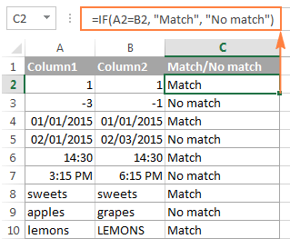
Example 2. Compare two lists for case-sensitive matches in the same row
As you have probably noticed, the formulas from the previous example ignore case when comparing text values, as in row 10 in the screenshot above. If you want to find case-sensitive matches between 2 columns in each row, then use the EXACT function:
=IF(EXACT(A2, B2), "Match", "")
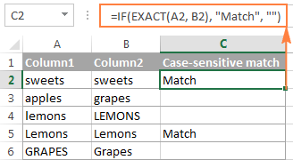
To find case-sensitive differences in the same row, enter the corresponding text ("Unique" in this example) in the 3rd argument of the IF function, e.g.:
=IF(EXACT(A2, B2), "Match", "Unique")
Compare multiple columns for matches in the same row
In your Excel worksheets, multiple columns can be compared based on the following criteria:
- Find rows with the same values in all columns (Example 1)
- Find rows with the same values in any 2 columns (Example 2)
Example 1. Find matches in all cells within the same row
If your table has three or more columns and you want to find rows that have the same values in all cells, an IF formula with an AND statement will work a treat:
=IF(AND(A2=B2, A2=C2), "Full match", "")
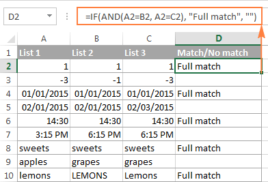
If your table has a lot of columns, a more elegant solution would be using the COUNTIF function:
=IF(COUNTIF($A2:$E2, $A2)=5, "Full match", "")
Where 5 is the number of columns you are comparing.
Example 2. Find matches in any two cells in the same row
If you are looking for a way to compare columns for any two or more cells with the same values within the same row, use an IF formula with an OR statement:
=IF(OR(A2=B2, B2=C2, A2=C2), "Match", "")
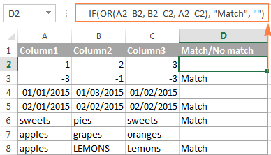
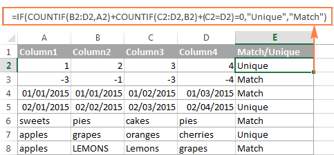
In case there are many columns to compare, your OR statement may grow too big in size. In this case, a better solution would be adding up several COUNTIF functions. The first COUNTIF counts how many columns have the same value as in the 1st column, the second COUNTIF counts how many of the remaining columns are equal to the 2nd column, and so on. If the count is 0, the formula returns "Unique", "Match" otherwise. For example:
=IF(COUNTIF(B2:D2,A2)+COUNTIF(C2:D2,B2)+(C2=D2)=0,"Unique","Match")
How to compare two columns in Excel for matches and differences
Suppose you have 2 lists of data in Excel, and you want to find all values (numbers, dates or text strings) which are in column A but not in column B.
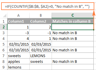
For this, you can embed the COUNTIF($B:$B, $A2)=0 function in IF's logical test and check if it returns zero (no match is found) or any other number (at least 1 match is found).
For instance, the following IF/COUNTIF formula searches across the entire column B for the value in cell A2. If no match is found, the formula returns "No match in B", an empty string otherwise:
=IF(COUNTIF($B:$B, $A2)=0, "No match in B", "")
Tip. If your table has a fixed number of rows, you can specify a certain range (e.g. $B2:$B10) rather than the entire column ($B:$B) for the formula to work faster on large data sets.
The same result can be achieved by using an IF formula with the embedded ISERROR and MATCH functions:
=IF(ISERROR(MATCH($A2,$B$2:$B$10,0)),"No match in B","")
Or, by using the following array formula (remember to press Ctrl + Shift + Enter to enter it correctly):
=IF(SUM(--($B$2:$B$10=$A2))=0, " No match in B", "")
If you want a single formula to identify both matches (duplicates) and differences (unique values), put some text for matches in the empty double quotes ("") in any of the above formulas. For example:
=IF(COUNTIF($B:$B, $A2)=0, "No match in B", "Match in B")
How to compare two lists in Excel and pull matches
Sometimes you may need not only match two columns in two different tables, but also pull matching entries from the lookup table. Microsoft Excel provides a special function for this - the VLOOKUP function. As an alternative, you can use a more powerful and versatile INDEX MATCH formula. The users of Excel 2021 and Excel 365, can accomplish the task with the XLOOKUP function.
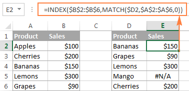
For example, the following formulas compare the product names in columns D against the names in column A and pull a corresponding sales figure from column B if a match is found, otherwise the #N/A error is returned.
=VLOOKUP(D2, $A$2:$B$6, 2, FALSE)
=INDEX($B$2:$B$6, MATCH($D2, $A$2:$A$6, 0))
=XLOOKUP(D2, $A$2:$A$6, $B$2:$B$6)
For more information, please see How to compare two columns using VLOOKUP.
If you don't feel very comfortable with formulas, you can have the job done using a fast and intuitive solution - Merge Tables Wizard.
Compare two lists and highlight matches and differences
When you compare columns in Excel, you may want to "visualize" the items that are present in one column but missing in the other. You can shade such cells in any color of your choosing by using the Excel Conditional Formatting feature and the following examples demonstrate the detailed steps.
Example 1. Highlight matches and differences in each row
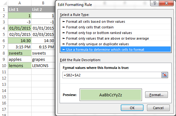
To compare two columns and Excel and highlight cells in column A that have identical entries in column B in the same row, do the following:
- Select the cells you want to highlight (you can select cells within one column or in several columns if you want to color entire rows).
- Click Conditional formatting > New Rule… > Use a formula to determine which cells to format.
- Create a rule with a simple formula like
=$B2=$A2(assuming that row 2 is the first row with data, not including the column header). Please double check that you use a relative row reference (without the $ sign) like in the formula above.
To highlight differences between column A and B, create a rule with this formula:
=$B2<>$A2
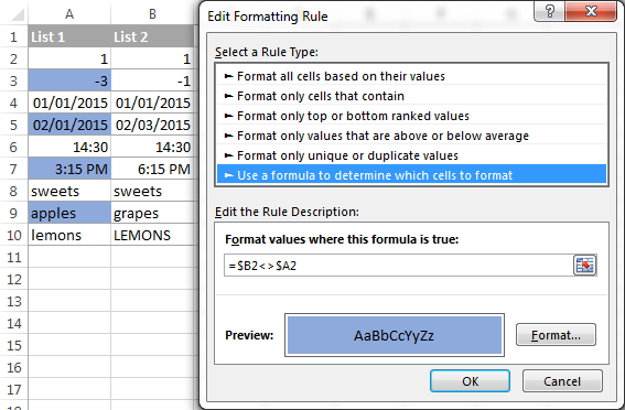
If you are new to Excel conditional formatting, please see How to create a formula-based conditional formatting rule for step-by-step instructions.
Example 2. Highlight unique entries in each list
Whenever you are comparing two lists in Excel, there are 3 item types that you can highlight:
- Items that are only in the 1st list (unique)
- Items that are only in the 2nd list (unique)
- Items that are in both lists (duplicates) - demonstrated in the next example.
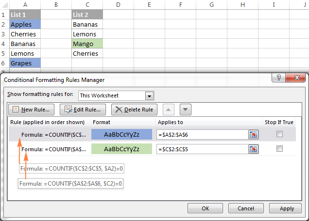
This example demonstrates how to color the items that are only in one list.
Supposing your List 1 is in column A (A2:A6) and List 2 in column C (C2:C5). You create the conditional formatting rules with the following formulas:
Highlight unique values in List 1 (column A):
=COUNTIF($C$2:$C$5, $A2)=0
Highlight unique values in List 2 (column C):
=COUNTIF($A$2:$A$6, $C2)=0
And get the following result:
Example 3. Highlight matches (duplicates) between 2 columns
If you closely followed the previous example, you won't have difficulties adjusting the COUNTIF formulas so that they find the matches rather than differences. All you have to do is to set the count greater than zero:
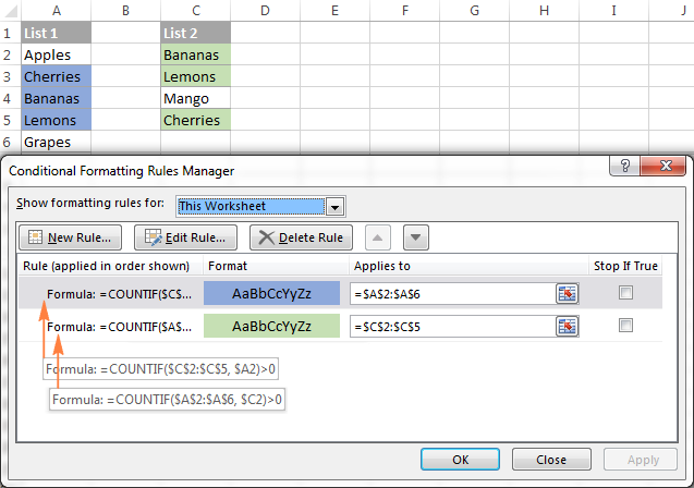
Highlight matches in List 1 (column A):
=COUNTIF($C$2:$C$5, $A2)>0
Highlight matches in List 2 (column C):
=COUNTIF($A$2:$A$6, $C2)>0
Highlight row differences and matches in multiple columns
When comparing values in several columns row-by-row, the quickest way to highlight matches is creating a conditional formatting rule, and the fastest way to shade differences is embracing the Go To Special feature, as demonstrated in the following examples.
Example 1. Compare multiple columns and highlight row matches
To highlight rows that have identical values in all columns, create a conditional formatting rule based on one of the following formulas:
=AND($A2=$B2, $A2=$C2)
or
=COUNTIF($A2:$C2, $A2)=3
Where A2, B2 and C2 are the top-most cells and 3 is the number of columns to compare.
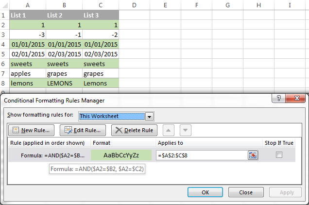
Of course, neither AND nor COUNTIF formula is limited to comparing only 3 columns, you can use similar formulas to highlight rows with the same values in 4, 5, 6 or more columns.
Example 2. Compare multiple columns and highlight row differences
To quickly highlight cells with different values in each individual row, you can use Excel's Go To Special feature.
- Select the range of cells you want to compare. In this example, I've selected cells A2 to C8.

By default, the top-most cell of the selected range is the active cell, and the cells from the other selected columns in the same row will be compared to that cell. As you can see in the screenshot above, the active cell is white while all other cells of the selected range are highlighted. In this example, the active cell is A2, so the comparison column is column A.
To change the comparison column, use either the Tab key to navigate through selected cells from left to right, or the Enter key to move from top to bottom.
Tip. To select non-adjacent columns, select the first column, press and hold Ctrl, and then select the other columns. The active cell will be in the last column (or in the last block of adjacent columns). To change the comparison column, use the Tab or Enter key as described above.
- On the Home tab, go to Editing group, and click Find & Select > Go To Special… Then select Row differences and click the OK button.
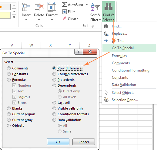
- The cells whose values are different from the comparison cell in each row are colored. If you want to shade the highlighted cells in some color, simply click the Fill Color icon on the ribbon and select the color of your choosing.

How to compare two cells in Excel
In fact, comparing 2 cells is a particular case of comparing two columns in Excel row-by-row except that you don't have to copy the formulas down to other cells in the column.
For example, to compare cells A1 and C1, you can use the following formulas.
For matches:
=IF(A1=C1, "Match", "")
For differences:
=IF(A1<>C1, "Difference", "")
To learn a few other ways to compare cells in Excel, please see:
Formula-free way to compare two columns / lists in Excel
Now that you know Excel's offerings for comparing and matching columns, let me show you our own solution for this task. This tool is named Compare Two Tables and it is included in our Ultimate Suite.
The add-in can compare two tables or lists by any number of columns and both identify matches/differences (as we did with formulas) and highlight them (as we did with conditional formatting).
For the purpose of this article, we'll be comparing the following 2 lists to find common values that are present in both.

To compare two lists, here are the steps you need to follow:
- Start with clicking the Compare Tables button on the Ablebits Data tab.

- Select the first column/list and click Next. In terms of the add-in, this is your Table 1.

- Select the second column/list and click Next. In terms of the add-in, it is your Table 2, and it can reside in the same or different worksheet or even in another workbook.

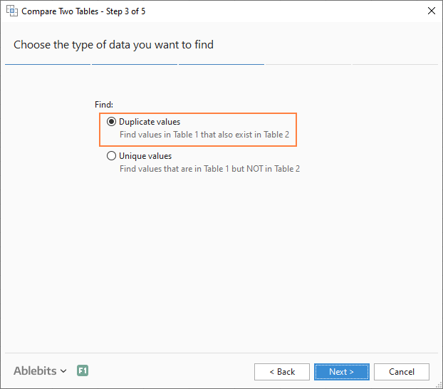
- Choose what kind of data to look for:
- Duplicate values (matches) - the items that exist in both lists.
- Unique values (differences) - the items that are present in list 1, but not in list 2.
Since our aim is to find matches, we select the first option and click Next.
- This is the key step where you select the columns for comparison. In our case, the choice is obvious as we are only comparing 2 columns: 2000 Winners against 2021 Winners. In bigger tables, you can select several column pairs to compare by.

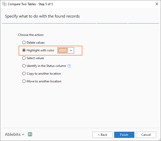
- In the final step, you choose how to deal with the found items and click Finish.
A few different options are available here. For our purposes, these two are most useful:
- Highlight with color - shades matches or differences in the selected color (like Excel conditional formatting does).
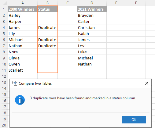
- Identify in the Status column - inserts the Status column with the "Duplicate" or "Unique" labels (like IF formulas do).
For this example, I've decided to highlight duplicates in the following color:
And in a moment, got the following result:

With the Status column, the result would look as follows:
Tip. If the lists you are comparing are in different worksheets or workbooks, it might be helpful to view Excel sheets side by side.
This is how you compare columns in Excel for matches (duplicates) and differences (unique values). If you are interested to try this tool, you are welcome to download an evaluation version using the below link.
I thank you for reading and encourage you to check out other helpful tutorials that we have :)
Available downloads
Compare Excel Lists - examples (.xlsx file)
Ultimate Suite - trial version (.exe file)
 by
by
550 comments
Hello,
I need help on this issue. I want to compare values of 2 columns. I want a visual marker that will highlight (or mark as a duplicate) as long as any value of one column is contained in the other column.
Hello.
I need help on this issue. I wan to compare values of 2 columns. These values, even though they same, are not necessarily arranged in same order or may not even be of same string, eg.
Jason Paul Macaulay Macaulay Paul
J P Macaulay Jason Paul Macaulay
Macaulay Jason Jason Paul Macaulay
Macaulay Paul J P Macaulay
Hello, I have been trying pull some matching data with little luck. I have 2 data sets 1 with demographic information and one with home sales information. Both have addresses I have broken down by: home number, direction,street name. These data sets are on 2 different sheets. How do I find matching: home number, direction, street name on each sheet? Hopefully that makes sense.
Hi,
Hopefully someone can understand what I am trying to do here.
I am currently going through some spreadsheet files and I would like to find case based non-duplicates e.g.
Column A Column B
Row 1 Harry Potter Ron Weasley
Row 2 harry potter Ron Weasley
Basically I am looking for true non-duplicates where the case of the text is concerned, the above example using the method I am currently using (Conditional formatting and Highlight duplicate values) will mark the above A1&A2 example as a duplicate even though the case being different, I would like a solution to mark the A1&A2 entry as a non duplicate by any visual method to differentiate from an actual true duplicate entry e.g. B1&B2, note I do not want to manipulate the data to become true duplicates just want to highlight the case differences.I'm cross examining two Rows with about 40-50 Columns, in a multitude of files.
Is what I am trying to achieve possible?
Any and all help will be appreciated.
Kind Regards
Jack
any feedback
Hi
I need to make filter for unique value that created by multi user once per month per user than we need to calculate the QTY of the unique number per user
Example for my Question:
transaction_date Value User_NAME
--------------------------------------------------
1/1/2017 1222889205 MarK
--------------------------------------------------
2/1/2017 1222889205 Mac
--------------------------------------------------
4/1/2017 1254879863 Eva
--------------------------------------------------
21/2/2017 1225478962 Jake
--------------------------------------------------
4/5/2017 1254879863 Eva
--------------------------------------------------
5/5/2017 1254879863 Eva
--------------------------------------------------
1/6/2017 1254793658 Mac
--------------------------------------------------
1/6/2017 1254793658 Jake
--------------------------------------------------
6/6/2017 1254793658 Eva
--------------------------------------------------
**my Solution
Month user Count for uniqe value
--------------------------------------------------
jan MarK 1
Mac 1
Eva 1
-----------------------------------------------
Feb JaKe 1
---------------------------------------------
May Eva 1
----------------------------------------------
Jun Mac 1
JaKe 1
Eva 1
---------------------------------------------
Appreciate your support thanks
I am facing an issue of 10,000 row items contains data for visits.
data contains same name but different start date and end date
Shop Name Opening End
CRUSH TRUCKING STATION 12-May-11 22-Dec-14
SUPERIOR II FILLING STATION 11-Dec-13 14-Mar-14
INDUS FILLING STATION 13-Dec-13 21-Feb-14
INDUS FILLING STATION 21-Feb-14 17-Oct-14
SUPERIOR II FILLING STATION 14-Mar-14 23-Oct-14
INDUS FILLING STATION 17-Oct-14 25-Jan-15
SUPERIOR II FILLING STATION 23-Oct-14 16-Jan-15
SUPERIOR II FILLING STATION 16-Jan-15 08-May-15
Is there any solution for above to adjust columns in start and end date in same shop name
I need some help.
I am using vlookup to draw information from sheets A and B and then compare them side by side on Sheet C. The values happen to be in time format. I need to have a formula (or a quick system) to highlight the the cells so that I can quickly spot the different in the times and then correct them. The spreadsheet that I am using is already full of useful conditional formatting and so would really like it to just appear a different colour so that it gets my attention.
Any suggestions much appreciated
Hi, I need to copy data from one cell to another on daily basis
Example,
A1 : =TODAY() //Changes Daily
B1 : =SUM(B2:B10) //Changes Daily
I need the B1 value to be copied on C1
Next day B1 value to be copied on C2
Next day B1 value to be copied on C3 and so on...
Waiting for your support
Thanks in advance
HELP!
Would you please help me?
It is really important.
What i want to do is this
compare columns for any two or more cells with the same values within the same row and hightlight individual rows after matching
I have 20 different columns that i need to compare for any two or more duplicate cells among them
How can i do that with the simplest way?
Thank you
Hello, Kostis,
Please try Duplicate Remover for Excel:
https://www.ablebits.com/excel-suite/find-remove-duplicates.php
You can run it on pairs of columns several times. Select the first column as master table and the second as your lookup table. You can email a sample table with your data in Excel to support@ablebits.com for more detailed instructions.
Hi,
I have an sheet with columns from January to December where people make contributions on monthly basis. A person's contribution is the same through out the year.
I would want a formula that shows if someone is contributing the same figure throughout the year or not, kind of like "True" and "False" formula but it should be checking in all the columns thus January-December and not just two columns whose formula I know is =A2=B2
Thanks.
not working the below formula in excel 2016, please guide if any changes on this?
=IF(COUNTIFS($CU2:$CU59862,CU2, $CA2:$CA59862,CA2, $FL2:$FL59862,FL2, $DA2:$DA59862,DA2, $DV2:$DV59862,DV2) >1, "DUPLICATE ROW","")
Excellent resource. I have two worksheets. one with 25,000 rows and the other with 63,000 rows and i want to find out the complete match of sheet2 to sheet 1, the ones without any match and others with at least 90% match. please how do i go about this. thank you
Hello I have 10 values in Col A and 3 values in Col B. I want to highlight only values that match col A with Col B and mark others in a diff color . How do i do it?
Col A Col B
1 1
2 6
3 9
4
5
6
7
8
9
10
Col A Col B
1 1 Match
2 No match
3 No match
4 No match
5 No match
6 6 match
7 No match
8 No match
9 9 match
10 No match
Hi, kindly help me derive a proper formula for this problem. I am using two sheets Sheet 1 & Sheet 2 in excel 2013. I created a drop down value (1-15 & 1-15) in the first sheet using data validation to derive two numbers in two different cells. In the second sheet I have created variables (with 1-15 in one cell and 1-15 in another cell) to derive a result in the third column). Say, in the first sheet I have one column no. of factories (1-15) & No of Managers (1-15). In the second sheet I have created the variable; No. of Factories, No of Manager & in the third row their Operating hours:
No of Factories: 1/2/3/4/5/....
No of Managers: 1/2/3/4/5/....
No of Operating hours: 8 (in case 1,1), 15 (1, 2), etc.
Now in the first sheet I want to use the drop down values to enter what i want to know and get the result using a formula.
Kindly help me with this.
how to Compare table columns in excel
for example
Table -1
Col A; Col B; Col C;
Roll No. Std. Name Result 1 semester (total Marks)
1 A 50
2 B 40
3 C 55
Table -2
Col A; Col B; Col C;
Roll No. Std. Name Result 2 semester (total Marks)
2 B 45
4 D 60
1 A 60
3 C 50
I Want to Result like that
Table -1 Table-2
Col A; Col B; Col C; Col D; Col E; Col F;
Roll No. Std. Name Result S-1 Roll No. Std. Name Result S-2
1 A 50 1 A 60
2 B 40 2 B 45
3 C 55 3 C 50
4 D 60
Could you described please how i could solve this as Table 2 match with table 1 and sort and place the record on same row
thanks
i want add the data with different uniqe item below following table
item data
1 4
2 3
1 2
3 2
2 3
1 1
Good day
I`m a marine engineer.I am just creating a worksheet where if a parameter in column F is greater than a parameter in columnn I by 0.03(P4>Pd>0.03),A separate column say H has to highlight each row as Abnormal with cell bgrnd as red.Would you please help me on this
Thanks in advance
Allan
I need help writing a formula to find matches between a column in SHEET1 and a column in SHEET2. Goal is to get "Match" inserted into Column B, SHEET1 if there is a match between Column A and Column B.
I tried:
=IF(A2=$SHEET2$,B2,"Match","") but this didn't work. Can someone help me out please!
Data:
Column A, SHEET1
12AB1250
12AB1251
12AB1252
Column A, SHEET2
12AB1250
12AB1251
12AB1252
12AB1253
12AB1254
12AB1255
Thanks in advance!
=IF(A2=A3,"Match","No match"
Copy and paste above formula and A1 delete and select Column A, SHEET1 and A3 delete and select Column A, SHEET2 . it will work
As a step in a bank reconciliation, I am comparing two list of $amt. I do have a unique identifier in one list but not the other, just $ values.
I want to compare the $values and find a "unique" match. Meaning, say I have $155 twice in list 1, three times in list 2.
Is there a way to id the match 2?
With a unique identifier in both list, two column match with condition formatting would work fine.
It a large volume of data, please help!