Is duplicate data in your worksheets causing you a headache? This tutorial will teach you how to quickly find, select, color or eliminate repeated entries in your dataset.
Whether you import data from an external source or collate it yourself, the duplication problem is the same - identical cells create a chaos in your spreadsheets, and you need to somehow deal with them. Since duplicates in Excel can take various forms, deduplication techniques may also vary. This tutorial brings into focus the most useful ones.
Note. This article shows how to search for duplicate cells in a range or list. If you are comparing two columns, then check out these solutions: How to find duplicates in 2 columns.
How to highlight duplicate cells in Excel
To highlight duplicate values in a column or range, you normally use Excel Conditional Formatting. In a simplest case, you can apply the predefined rule; in more sophisticated scenarios, you will have to create your own rule based on formula. The below examples illustrate both cases.
Example 1. Highlight duplicate cells including first occurrences
In this example, we will be using a preset rule available in all versions of Excel. As you can understand from the heading, this rule highlights all occurrences of a duplicate value, including the first one.
To apply the built-in rule for duplicates, perform these steps:
- Select a range where you want to find duplicate cells.
- On the Home tab, in the Styles group, click Conditional Formatting > Highlight Cells Rules > Duplicate Values…
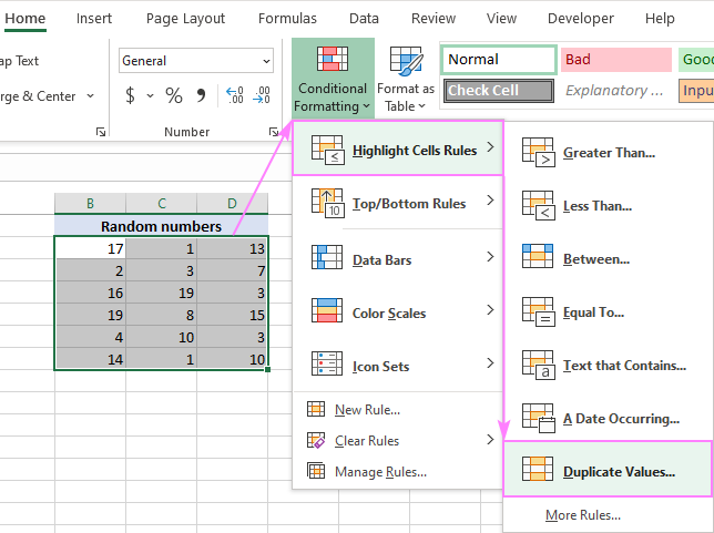
- In the Duplicate Values pop-up dialog, choose formatting for Duplicate cells (the default is Light Red Fill and Dark Red Text). Excel will show you a preview of the selected format right away, and if you are happy with it, click OK.

Tips:
- To apply your own formatting for duplicates, click Custom Format… (the last item in the drop-down list), and then choose the desired Font, Border and Fill options.
- To highlight unique cells, pick Unique in the left-hand box.
Example 2. Highlight duplicate cells except first occurrences
To mark duplicate values except 1st instances, the inbuilt rule cannot help, and you'll need to set up your own rule with a formula. The formula is quite tricky and requires adding a blank column to the left of your dataset (column A in this example).
To create a rule, these are the steps to perform:
- Select the target range.
- On the Home tab, in the Styles group, click Conditional Formatting > New rule > Use a formula to determine which cells to format.
- In the Format values where this formula is true box, enter the following formula:
=IF(COLUMNS($B2:B2)>1, COUNTIF(A$2:$B$7,B2),0) + COUNTIF(B$2:B2,B2)>1Where B2 is the first cell in the first column, B7 is the last cell in the first column, and A2 is the cell in the blank column corresponding to the first row in your selected range. The detailed explanation of the formula is provided in a separate tutorial.
- Click the Format… button and choose the formatting options you like.
- Click OK to save the rule.

Tips and notes:
- Example 2 requires an empty column to the left of the target range. If such a column cannot be added in your worksheet, then you can configure two different rules (one for the first column and another for all subsequent columns). The detailed instructions are provided here: Highlighting duplicates in multiple columns without 1st occurrences.
- The above solutions are for individual cells. If you are working with structured data, then see how to highlight rows based on duplicate values in a key column.
- A much easier way to highlight identical cells with or without 1st instances is by using the Find Duplicate Cells tool.
A lot more use cases and examples can be found in this tutorial: How to highlight duplicates in Excel.
How to find duplicate cells in Excel using formulas
When working with a column of values, you can easily identify duplicate cells with the help of the COUNTIF and IF functions.
To find duplicates including 1st occurrences, the generic formula is:
To spot duplicates excluding 1st occurrences, the general formula is:
As you can see, the formulas are very much alike, the difference is in how you define the source range.
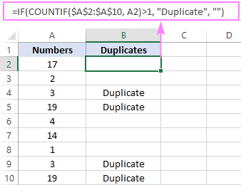
To locate duplicate cells including first instances, you compare the target cell (A2) with all other cells in the range $A$2:$A$10 (notice that we lock the range with absolute references), and if more than one cell containing same value are found, label the target cell as "Duplicate".
=IF(COUNTIF($A$2:$A$10, A2)>1, "Duplicate", "")
This formula goes to B2, and then you copy it down to as many cells as there are items in the list.
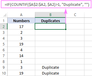
To get duplicate cells without first instances, you compare the target cell (A2) only with the above cells, not with each other cell in the range. For this, build an expanding range reference like $A$2:$A2.
=IF(COUNTIF($A$2:$A2, $A2)>1, "Duplicate", "")
When copied to the below cells, the range reference expands by 1. So, the formula in B2 compares the value in A2 only against this cell itself. In B3, the range expands to $A$2:$A3, so the value in A3 is compared against the above cell as well, and so on.
Tips:
- In this example, we were dealing with duplicate numbers. For text values, the formulas are exactly the same :)
- Once dupes are identified, you can turn on Excel Filter to display only repeated values. And then, you can do everything you want with the filtered cells: select, highlight, delete, copy or move to a new sheet.
For more formula examples, please see How to find duplicates in Excel.
How to delete duplicates in Excel
As you probably know, all modem versions of Excel are equipped with the Remove Duplicate tool, which works with the following caveats:
- It deletes entire rows based on duplicate values in one or more columns that you specify.
- It does not remove first occurrences of repeated values.
To remove duplicate records, this is what you need to do:
- Select the dataset you want to dedupe.
- On the Data tab, in the Data Tools group, click Remove Duplicates.
- In the Remove Duplicates dialog box, select the columns to check for dupes, and click OK.
In the below example, we want to check the first four columns for duplicates, so we select them. The Comments column is not really important and therefore is not selected.
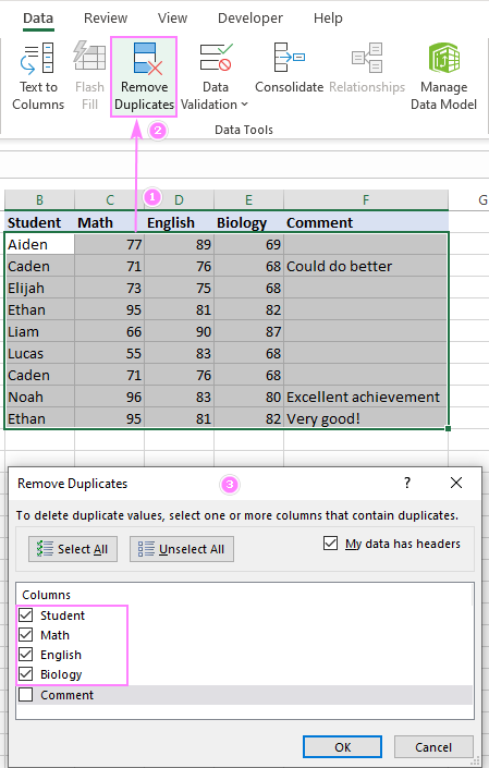
Based on the values in the selected columns, Excel has found and removed 2 duplicate records (for Caden and Ethan). The first instances of these records are retained.
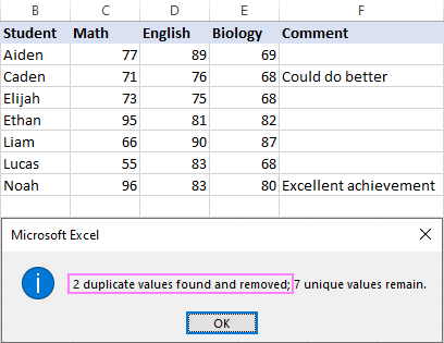
Tips:
- Before running the tool, it stands to reason to make a copy of your worksheet, so you don't lose any information if something goes wrong.
- Before attempting to eliminate duplicates, remove any filters, outlines or subtotals from your data.
- To delete duplicates in individual cells (like in the Randon numbers dataset from the very first example), use the Duplicate Cells tool discussed in the next example.
More use cases are covered in How to remove duplicate rows in Excel.
All-in-one tool to find and remove duplicate cells in Excel
As shown in the first part of this tutorial, Microsoft Excel provides a few different features to deal with duplicates. The problem is you need to know where to look for them and how to leverage them for your specific tasks.
To make the lives of our Ultimate Suite users easier, we have created a special tool to handle duplicate cells an easy way. Precisely what can it do? Almost everything you can think of :)
- Find duplicate cells (with or without 1st occurrences) or unique cells.
- Find cells with the same values, formulas, background or font color.
- Search for duplicate cells considering text case (case-sensitive search) and ignoring blanks.
- Clear duplicate cells (contents, formats or all).
- Color duplicate cells.
- Select duplicate cells.
Please let me introduce to you our recent addition to the Ablebits Duplicate Remover toolkit - Find Duplicate Cells add-in.
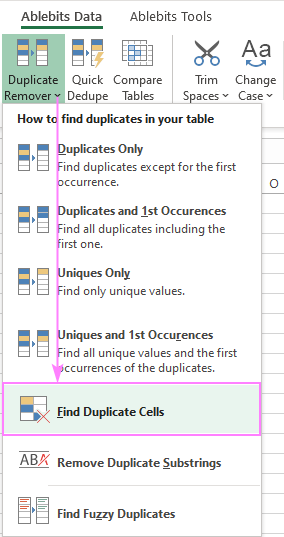
To find duplicates cells in your worksheet, carry out these steps:
- Select your data.
- On the Ablebits Data tab, click Duplicate Remover > Find Duplicate Cells.
- Choose whether to search for duplicate or unique cells.

- Specify whether to compare values, formulas or formatting and select the additional options if needed. The screenshot below shows the default settings:

- Finally, decide what to do with found duplicates: clear, highlight or simply select, and click Finish.

In this example, we've chosen to color duplicate cells except 1st occurrences and got the following result:
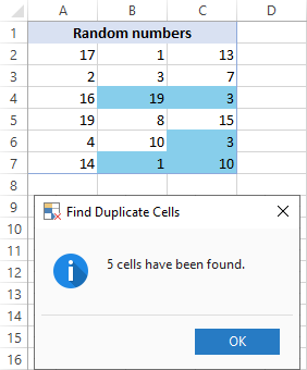
Remember that cumbersome formula for conditional formatting to achieve the same effect? ;)
If you are analyzing structured data organized in a table, then use Duplicate Remover to search for duplicates based on values in one or more columns.
To find duplicates in 2 columns or 2 different tables, run the Compare Two Tables tool.
The good news is that all these tools are included in Ultimate Suite and you can try any of them in your worksheets right now - the download link is right below.
I thank you for reading and hope to see you on our blog next week!
Available downloads
Find duplicate cells - examples (.xlsx file)
Ultimate Suite - trial version (.exe file)
 by
by
2 comments
Hello, I badly need your help. Obviously in ColumnA (Name) are duplicate names which I already conditionally formatted. But I need those results reflected in column C without copying repeated numbers from Column B (Study Room) is that even visible without thinking too much in VBA and other too conflict formulas? Hope its clear? Thanks!
Name Study Room Results
Clara 16 16
Clara 16
Jessica 12 10, 12
Jessica 10
Jessica 10
Jessica 12
Hello!
You can find the examples and detailed instructions here: Filter unique values based on multiple criteria.
The formula might look like this:
=TEXTJOIN(", ",TRUE,UNIQUE(FILTER(B1:B10,A1:A10=A1)))
To merge values in a single cell, use the TEXTJOIN function.