The tutorial shows how to use VLOOKUP formula in Excel to compare two columns to return common values (matches) or find missing data (differences).
When you have data in two different lists, you may often need to compare them to see what information is missing in one of the lists or what data is present in both. Comparison can be done in many different ways - which method to use depends on exactly what you want from it.
How to compare two columns in Excel using VLOOKUP
When you have two columns of data and want to find out which data points from one list exist in the other list, you can use the VLOOKUP function to compare the lists for common values.
To build a VLOOKUP formula in its basic form, this is what you need to do:
- For lookup_value (1st argument), use the topmost cell from List 1.
- For table_array (2nd argument), supply the entire List 2.
- For col_index_num (3rd argument), use 1 as there is just one column in the array.
- For range_lookup (4th argument), set FALSE - exact match.
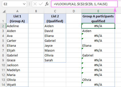
Suppose you have the names of participants in column A (List 1) and the names of those who have passed through the qualification rounds in column B (List 2). You want to compare these 2 lists to determine which participants from Group A made their way to the main event. To do this, use the following formula.
=VLOOKUP(A2, $C$2:$C$9, 1, FALSE)
The formula goes to cell E2, and then you drag it down through as many cells as there are items in List 1.
Please notice that table_array is locked with absolute references ($C$2:$C$9) so that it remains constant when you copy the formula to the below cells.
As you can see, the names of the qualified athletes show up in column E. For the remaining participants, a #N/A error appears indicating that their names are not available in List 2.

Disguise #N/A errors
The VLOOKUP formula discussed above perfectly fulfills its main objective - returns common values and identifies missing data points. However, it delivers a bunch of #N/A errors, which may confuse inexperienced users making them think that something is wrong with the formula.
To replace errors with blank cells, use VLOOKUP in combination with the IFNA or IFERROR function in this way:
=IFNA(VLOOKUP(A2, $C$2:$C$9, 1, FALSE), "")

Our improved formula returns an empty string ("") instead of #N/A. You can also return your custom text such as "Not in List 2", "Not present", or "Not available". For example:
=IFNA(VLOOKUP(A2, $C$2:$C$9, 1, FALSE), "Not in List 2")
That is the basic VLOOKUP formula to compare two columns in Excel. Depending on your particular task, it can be modified as shown in further examples.
Compare two columns in different Excel sheets using VLOOKUP
In real life, the columns you need to compare are not always on the same sheet. In a small dataset, you can try spotting the differences manually by viewing two sheets side by side.
To search in another worksheet or workbook with formulas, you have to use external reference. The best practice is to start typing the formula in your main sheet, then switch to the other worksheet and select the list using the mouse - an appropriate range reference will be added to the formula automatically.
Assuming List 1 is in column A on Sheet1 and list 2 is in column A on Sheet2, you can compare two columns and find matches using this formula:
=IFNA(VLOOKUP(A2, Sheet2!$A$2:$A$9, 1, FALSE), "")

For more information, please see:
Compare two columns and return common values (matches)
In the previous examples, we discussed a VLOOKUP formula in its simplest form:
=IFNA(VLOOKUP(A2, $C$2:$C$9, 1, FALSE), "")
The result of that formula is a list of values that exist in both columns and blank cells in place of the values not available in the second column.
To get a list of common values without gaps, just add auto-filter to the resulting column and filter out blanks.

In Excel for Microsoft 365 and Excel 2021 that support dynamic arrays, you can make use of the FILTER function to sift out blanks dynamically. For this, utilize the IFNA VLOOKUP formula as the criteria for FILTER:
=FILTER(A2:A14, IFNA(VLOOKUP(A2:A14, C2:C9, 1, FALSE), "")<>"")
Please pay attention that in this case we supply the entire List 1 (A2:A14) to the lookup_value argument of VLOOKUP. The function compares each of the lookup values against List 2 (C2:C9) and returns an array of matches and #N/A errors representing missing values. The IFNA function replaces errors with empty strings and serves the results to the FILTER function, which filters out blanks (<>"") and outputs an array of matches as the final result.

Alternatively, you can use the ISNA function to check the result of VLOOKUP and filter the items evaluating to FALSE, i.e. values other than #N/A errors:
=FILTER(A2:A14, ISNA(VLOOKUP(A2:A14, C2:C9, 1, FALSE))=FALSE)
The same result can be achieved with the XLOOKUP function, which makes the formula even simpler. Due to the ability of XLOOKUP to handle #N/A errors internally (optional if_not_found argument), we can do without the IFNA or ISNA wrapper:
=FILTER(A2:A14, XLOOKUP(A2:A14, C2:C9, C2:C9,"")<>"")
Compare two columns and find missing values (differences)
To compare 2 columns in Excel to find differences, you can proceed in this way:
- Write the core formula to search for the first value from List 1 (A2) in List 2 ($C$2:$C$9):
VLOOKUP(A2, $C$2:$C$9, 1, FALSE)
- Nest the above formula in the ISNA function to check the VLOOKUP's output for #N/A errors. In case of an error, ISNA yields TRUE, otherwise FALSE:
ISNA(VLOOKUP(A2, $C$2:$C$9, 1, FALSE))
- Use the ISNA VLOOKUP formula for the logical test of the IF function. If the test evaluates to TRUE (#N/A error), return a value from List 1 in the same row. If the test evaluates to FALSE (a match in List 2 is found), return an empty string.
The complete formula takes this form:
=IF(ISNA(VLOOKUP(A2, $C$2:$C$9, 1, FALSE)), A2, "")
To get rid of the blanks, apply Excel's Filter as demonstrated in the above example.

In Excel 365 and Excel 2021, you can have the result list filtered dynamically. For this, simply place the ISNA VLOOKUP formula in the include argument of the FILTER function:
=FILTER(A2:A14, ISNA(VLOOKUP(A2:A14, C2:C9, 1, FALSE)))

Another way is to use XLOOKUP for criteria - the function returns empty strings ("") for missing data points, and you filter the values in List 1 for which XLOOKUP returned empty strings (=""):
=FILTER(A2:A14, XLOOKUP(A2:A14, C2:C9, C2:C9,"")="")
VLOOKUP formula to identify matches and differences between two columns
If you want to add text labels to the first list indicating which values are available in the second list and which are not, use the VLOOKUP formula together with the IF and ISNA/ISERROR functions.
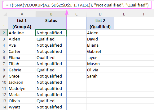
For example, to identify names that are in both columns A and D and those that are only in column A, the formula is:
=IF(ISNA(VLOOKUP(A2, $D$2:$D$9, 1, FALSE)), "Not qualified", "Qualified")
Here, the ISNA function catches the #N/A errors generated by VLOOKUP and passes that intermediate result to the IF function for it to return the specified text for errors and another text for successful lookups.
In this example, we used "Not qualified"/"Qualified" labels, which are suitable for our sample dataset. You can replace them with "Not in List 2"/"In List 2", "Not available"/"Available" or any other labels you see fit.
This formula is best to be inserted in a column adjacent to List 1 and copied through as many cells as there are items in your list.

One more way to identify matches and differences in 2 columns is using the MATCH function:
=IF(ISNA(MATCH(A2, $D$2:$D$9, 0)), "Not in List 2", "In List 2")

A few other ways to accomplish the task are described in this tutorial: Check if value exists in a range.
Compare 2 columns and return a value from third
When working with tables containing related data, you may sometimes need to compare two columns in two different tables and return a matching value from another column. In fact, it is the primary use of the VLOOKUP function, the purpose it was designed for.
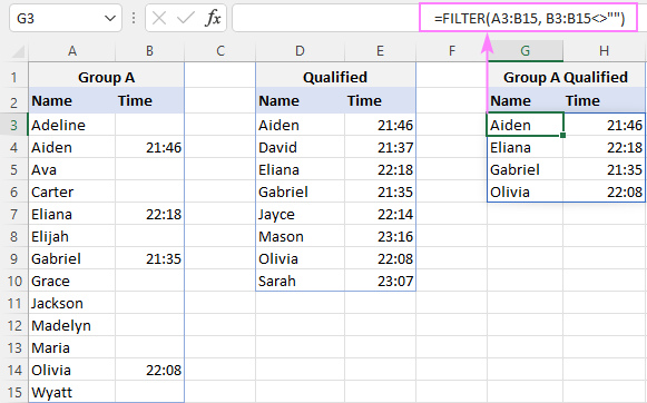
For example, to compare the names in columns A and D in the two tables below and return a time from column E, the formula is:
=VLOOKUP(A3, $D$3:$E$10, 2, FALSE)

To hide #N/A errors, use the proven solution - the IFNA function:
=IFNA(VLOOKUP(A3, $D$3:$E$10, 2, FALSE), "")

Instead of blanks, you can return any text you want for missing data points - just type it in the last argument. For instance:
=IFNA(VLOOKUP(A3, $D$3:$E$10, 2, FALSE), "Not available")
Besides VLOOKUP, the task can be fulfilled with a few other lookup functions.
Personally, I'd rely on a more flexible INDEX MATCH formula:
=IFNA(INDEX($E$3:$E$10, MATCH(A3, $D$3:$D$10, 0)), "")
Or use the modern successor of VLOOKUP - the XLOOKUP function, available in Excel 365 and Excel 2021:
=XLOOKUP(A3, $D$3:$D$10, $E$3:$E$10, "")
To get the names of qualified participants from group A and their results, simply filter out blank cells in column B:
=FILTER(A3:B15, B3:B15<>"")

Comparison tools
If you frequently do file or data comparison in Excel, these smart tools included in our Ultimate Suite can save your time immensely!
Compare Tables - quick way to find duplicates (matches) and unique values (differences) in any two data sets such as columns, list or tables.
Compare Two Sheets - find and highlight differences between two worksheets.
Compare Multiple Sheets - find and highlight differences in multiple sheets at once.
Practice workbook for download
VLOOKUP in Excel to compare columns - examples (.xlsx file)
 by
by
16 comments
Hi, I've got my results from the following formula that you provided. =IF(ISNA(VLOOKUP('HPY_PAID REPORT'!M2,'Regular HOURS'!A:F,1,FALSE)), 'HPY_PAID REPORT'!M2, "") but now I would like to "remove duplicates" automatically from the results from the =IF formula.
I know how to do it manually, but how am I able to insert it into the formula
Hi! This formula is not an array formula. It must be copied into the cells below the column. These instructions will allow you to extract a list of unique values from this column: How to get a list of unique and distinct values in Excel and Excel UNIQUE function - fastest way to find unique values.
Hi,
I have two Excel sheets (Sheet 1 and Sheet 2) with two columns for first and last name. The data in Sheet 2 shows the same information as Sheet 1, however two people are missing. I compared them by the last name, however it brought three missing results since one of the people in Sheet 2 has changed only their last name.
How can I bring only the two missing people?
Hi! If I understand your task correctly, the following tutorial should help: Compare multiple columns for matches in the same row.
You can compare two tables without using formulas using Compare Two Tables tool. It is available as a part of our Ultimate Suite for Excel that you can install in a trial mode and check how it works for free.
Hi there,
I need some help on how to calculate hours for a client. There are two clients here, each with more than one CancelDescriptions. How can I add hours altogether for each client with data from multiple columns with Cells like this for example
A B C D E F
Client Duration CancelDescription
Sam 7 Public Holiday
Sam 4 Staff Leave
Sam 5.5 Blanks
Sam 3 Family unavailable
Paul 4.5 Staff Leave
Paul 2.5 Blanks
Also what formula to use if new client is added to the Sheet
Hi!
If I understand the problem correctly, you can calculate the amount of hours for each customer using the SUMIFS function.
=SUMIFS(B2:B9, A2:A9, "Sam")
=SUMIFS(C2:C9, A2:A9, A2)
I hope it’ll be helpful. If something is still unclear, please feel free to ask.
I have some data, A column is a persons name and the same name can appear multiple times, B column is a year and then C column is data that relates to that year. How can i use VLOOKUP to squish up column a without losing the data from column B&C?
Hello!
Here is the article that may be helpful to you: Vlookup multiple matches in Excel with one or more criteria. If you want to merge results in one cell, use the TEXTJOIN function.
I hope it’ll be helpful.
hi
please advise... i have a chart of pipe weight / meter as per their size (dia) and schedule number categories. it can be found on google easily. in first column (category1) it has pipes with dia 1", 2" and in first row (category2) it has schedule data e.g. sch10, sch.40 and in the middle area it has the corresponding values of weight e.g. for pipe dia 1" sch10 w/m is 2.09, for pipe dia 1" sch40 w/m is 2.5, for pipe dia 2" sch10 w/m is 3.93, for pipe dia 2" sch40 w/m is 5.44.
i want to make a sheet where i just select the pipe size and it's schedule and the weight / meter (w/m) shows accordingly.
Regards
Waseem Akram
Hello!
Try to use the examples and recommendations described in this article: Excel INDEX MATCH with multiple criteria. This should solve your task.
If i wanted to highlight similar text Eg; Column 1 has Luis and column 2 has Luis B and i want to highlight them both because there similar? How would i go about this?
Hello!
You can use conditional formatting to change a color of similar cells with the formula:
=ISNUMBER(SEARCH(A1,B1))+ISNUMBER(SEARCH(B1,A1))
The SEARCH function searches within text. ISNUMBER returns TRUE if the lookup was successful.
I hope my advice will help you solve your task.
Not quite working. Allow me to rephrase to avoid confusion.
I have 2 columns that run at least a hundred rows.
First column has text names on it, (EG; Luis)
Second column also has text names, (Eg; Luis B) but are not identical and need to be parsed out so I can highlight each text name on each column that has similarities?
Hi!
This formula will help you determine if a similar value exists in column B.
=SUM(--ISNUMBER(SEARCH(A1,B1:B10)))
Fuzzy Duplicates Finder can also help you determine fuzzy matches. It is available as a part of our Ultimate Suite for Excel that you can install in a trial mode and check how it works for free.
Hii
In sheet 1, column C (Owner Names) and Column D (Tenant names) are provided along with "Comments" in Column E for a city. And in sheet 2, owner names are provided in column F, and tenant names are in Column H, but comments are not provided.
Now I want, if in sheet1, any of the rows, the Owner name and tenant name exactly match with the owner's name and tenant name in Sheet2 . then the comments should be copied from sheet 1 to sheet 2 in column O. In other words, if Column C & Column D (Sheet1) = Column F & Column H (Sheet 2), then from sheet 1 column E (Comments) should be pasted in Column O in the sheet 2.
Hope I mentioned my problem correctly, please help me to generate the formula for this.
Hello!
You can find the examples and detailed instructions here: Excel INDEX MATCH with multiple criteria. You will be able to extract a value based on two criteria.