The tutorial provides a list of Excel basic formulas and functions with examples and links to related in-depth tutorials.
Being primarily designed as a spreadsheet program, Microsoft Excel is extremely powerful and versatile when it comes to calculating numbers or solving math and engineering problems. It enables you to total or average a column of numbers in the blink of an eye. Apart from that, you can compute a compound interest and weighted average, get the optimal budget for your advertising campaign, minimize the shipment costs or make the optimal work schedule for your employees. All this is done by entering formulas in cells.
This tutorial aims to teach you the essentials of Excel functions and show how to use basic formulas in Excel.
The basics of Excel formulas
Before providing the basic Excel formulas list, let's define the key terms just to make sure we are on the same page. So, what do we call an Excel formula and Excel function?
- Formula is an expression that calculates values in a cell or in a range of cells.
For example,
=A2+A2+A3+A4is a formula that adds up the values in cells A2 through A4. - Function is a predefined formula already available in Excel. Functions perform specific calculations in a particular order based on the specified values, called arguments, or parameters.
For example, instead of specifying each value to be summed like in the above formula, you can use the SUM function to add up a range of cells: =SUM(A2:A4)
You can find all available Excel functions in the Function Library on the Formulas tab:

There exist 400+ functions in Excel, and the number is growing by version to version. Of course, it's next to impossible to memorize all of them, and you actually don't need to. The Function Wizard will help you find the function best suited for a particular task, while the Excel Formula Intellisense will prompt the function's syntax and arguments as soon as you type the function's name preceded by an equal sign in a cell:
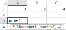
Clicking the function's name will turn it into a blue hyperlink, which will open the Help topic for that function.
Tip. You don't necessarily have to type a function name in all caps, Microsoft Excel will automatically capitalize it once you finish typing the formula and press the Enter key to complete it.
10 Excel basic functions you should definitely know
What follows below is a list of 10 simple yet really helpful functions that are a necessary skill for everyone who wishes to turn from an Excel novice to an Excel professional.
SUM
The first Excel function you should be familiar with is the one that performs the basic arithmetic operation of addition:
In the syntax of all Excel functions, an argument enclosed in [square brackets] is optional, other arguments are required. Meaning, your Sum formula should include at least 1 number, reference to a cell or a range of cells. For example:
=SUM(B2:B6) - adds up values in cells B2 through B6.
=SUM(B2, B6) - adds up values in cells B2 and B6.
If necessary, you can perform other calculations within a single formula, for example, add up values in cells B2 through B6, and then divide the sum by 5:
=SUM(B2:B6)/5
To sum with conditions, use the SUMIF function: in the 1st argument, you enter the range of cells to be tested against the criteria (A2:A6), in the 2nd argument - the criteria itself (D2), and in the last argument - the cells to sum (B2:B6):
=SUMIF(A2:A6, D2, B2:B6)
In your Excel worksheets, the formulas may look something similar to this:

Tip. The fastest way to sum a column or row of numbers is to select a cell next to the numbers you want to sum (the cell immediately below the last value in the column or to the right of the last number in the row), and click the AutoSum button on the Home tab, in the Formats group. Excel will insert a SUM formula for you automatically.
Useful resources:
AVERAGE
The Excel AVERAGE function does exactly what its name suggests, i.e. finds an average, or arithmetic mean, of numbers. Its syntax is similar to SUM's:
Having a closer look at the formula from the previous section (=SUM(B2:B6)/5), what does it actually do? Sums values in cells B2 through B6, and then divides the result by 5. And what do you call adding up a group of numbers and then dividing the sum by the count of those numbers? Yep, an average!
The Excel AVERAGE function performs these calculations behind the scenes. So, instead of dividing sum by count, you can simply put this formula in a cell:
=AVERAGE(B2:B6)
To average cells based on condition, use the following AVERAGEIF formula, where A2:A6 is the criteria range, D3 is he criteria, and B2:B6 are the cells to average:
=AVERAGEIF(A2:A6, D3, B2:B6)

Useful resources:
MAX & MIN
The MAX and MIN formulas in Excel get the largest and smallest value in a set of numbers, respectively. For our sample data set, the formulas will be as simple as:
=MAX(B2:B6)
=MIN(B2:B6)

Useful resources:
COUNT & COUNTA
If you are curious to know how many cells in a given range contain numeric values (numbers or dates), don't waste your time counting them by hand. The Excel COUNT function will bring you the count in a heartbeat:
While the COUNT function deals only with those cells that contain numbers, the COUNTA function counts all cells that are not blank, whether they contain numbers, dates, times, text, logical values of TRUE and FALSE, errors or empty text strings (""):
For example, to find out how many cells in column B contain numbers, use this formula:
=COUNT(B:B)
To count all non-empty cells in column B, go with this one:
=COUNTA(B:B)
In both formulas, you use the so-called "whole column reference" (B:B) that refers to all the cells within column B.
The following screenshot shows the difference: while COUNT processes only numbers, COUNTA outputs the total number of non-blank cells in column B, including the the text value in the column header.

Useful resources:
IF
Judging by the number of IF-related comments on our blog, it's the most popular function in Excel. In simple terms, you use an IF formula to ask Excel to test a certain condition and return one value or perform one calculation if the condition is met, and another value or calculation if the condition is not met:
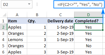
For example, the following IF statement checks if the order is completed (i.e. there is a value in column C) or not. To test if a cell is not blank, you use the "not equal to" operator ( <>) in combination with an empty string (""). As the result, if cell C2 is not empty, the formula returns "Yes", otherwise "No":
=IF(C2<>"", "Yes", "No")
Useful resources:
TRIM
If your obviously correct Excel formulas return just a bunch of errors, one of the first things to check is extra spaces in the referenced cells (You may be surprised to know how many leading, trailing and in-between spaces lurk unnoticed in your sheets just until something goes wrong!).
There are several ways to remove unwanted spaces in Excel, with the TRIM function being the easiest one:
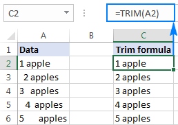
For example, to trim extra spaces in column A, enter the following formula in cell A1, and then copy it down the column:
=TRIM(A1)
It will eliminate all extra spaces in cells but a single space character between words:
Useful resources:
LEN
Whenever you want to know the number of characters in a certain cell, LEN is the function to use:
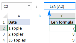
Wish to find out how many characters are in cell A2? Just type the below formula into another cell:
=LEN(A2)
Please keep in mind that the Excel LEN function counts absolutely all characters including spaces:
Want to get the total count of characters in a range or cells or count only specific characters? Please check out the following resources.
Useful resources:
AND & OR
These are the two most popular logical functions to check multiple criteria. The difference is how they do this:
- AND returns TRUE if all conditions are met, FALSE otherwise.
- OR returns TRUE if any condition is met, FALSE otherwise.
While rarely used on their own, these functions come in very handy as part of bigger formulas.
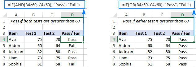
For example, to check the test results in columns B and C and return "Pass" if both are greater than 60, "Fail" otherwise, use the following IF formula with an embedded AND statement:
=IF(AND(B2>60, B2>60), "Pass", "Fail")
If it's sufficient to have just one test score greater than 60 (either test 1 or test 2), embed the OR statement:
=IF(OR(B2>60, B2>60), "Pass", "Fail")
Useful resources:
CONCATENATE
In case you want to take values from two or more cells and combine them into one cell, use the concatenate operator (&) or the CONCATENATE function:
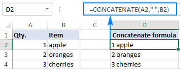
For example, to combine the values from cells A2 and B2, just enter the following formula in a different cell:
=CONCATENATE(A2, B2)
To separate the combined values with a space, type the space character (" ") in the arguments list:
=CONCATENATE(A2, " ", B2)
Useful resources:
TODAY & NOW
To see the current date and time whenever you open your worksheet without having to manually update it on a daily basis, use either:
=TODAY() to insert the today's date in a cell.
=NOW() to insert the current date and time in a cell.
The beauty of these functions is that they don't require any arguments at all, you type the formulas exactly as written above.

Useful resources:
Best practices for writing Excel formulas
Now that you are familiar with the basic Excel formulas, these tips will give you some guidance on how to use them most effectively and avoid common formula errors.
Do not enclose numbers in double quotes
Any text included in your Excel formulas should be enclosed in "quotation marks". However, you should never do that to numbers, unless you want Excel to treat them as text values.
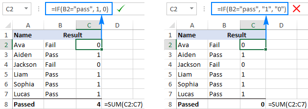
For example, to check the value in cell B2 and return 1 for "Passed", 0 otherwise, you put the following formula, say, in C2:
=IF(B2="pass", 1, 0)
Copy the formula down to other cells and you will have a column of 1's and 0's that can be calculated without a hitch.
Now, see what happens if you double quote the numbers:
=IF(B2="pass", "1", "0")
At first sight, the output is normal - the same column of 1's and 0's. Upon a closer look, however, you will notice that the resulting values are left-aligned in cells by default, meaning those are numeric strings, not numbers! If later on someone will try to calculate those 1's and 0's, they might end up pulling their hair out trying to figure out why a 100% correct Sum or Count formula returns nothing but zero.
Don't format numbers in Excel formulas
Please remember this simple rule: numbers supplied to your Excel formulas should be entered without any formatting like decimal separator or dollar sign. In North America and some other countries, comma is the default argument separator, and the dollar sign ($) is used to make absolute cell references. Using those characters in numbers may just drive your Excel crazy :) So, instead of typing $2,000, simply type 2000, and then format the output value to your liking by setting up a custom Excel number format.
Match all opening and closing parentheses
When crating a complex Excel formula with one or more nested functions, you will have to use more than one set of parentheses to define the order of calculations. In such formulas, be sure to pair the parentheses properly so that there is a closing parenthesis for every opening parenthesis. To make the job easier for you, Excel shades parenthesis pairs in different colors when you enter or edit a formula.
Copy the same formula to other cells instead of re-typing it
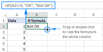
Once you have typed a formula into a cell, there is no need to re-type it over and over again. Simply copy the formula to adjacent cells by dragging the fill handle (a small square at the lower right-hand corner of the cell). To copy the formula to the whole column, position the mouse pointer to the fill handle and double-click the plus sign.
Note. After copying the formula, make sure that all cell references are correct. Cell references may change depending on whether they are absolute (do not change) or relative (change).
For the detailed step-by-step instructions, please see How to copy formulas in Excel.
How to delete formula, but keep calculated value
When you remove a formula by pressing the Delete key, a calculated value is also deleted. However, you can delete only the formula and keep the resulting value in the cell. Here's how:
- Select all cells with your formulas.
- Press Ctrl + C to copy the selected cells.
- Right-click the selection, and then click Paste Values > Values to paste the calculated values back to the selected cells. Or, press the Paste Special shortcut: Shift+F10 and then V.
For the detailed steps with screenshots, please see How to replace formulas with their values in Excel.
Make sure Calculation Options are set to Automatic
If all of a sudden your Excel formulas have stopped recalculating automatically, most likely the Calculation Options somehow switched to Manual. To fix this, go to the Formulas tab > Calculation group, click the Calculation Options button, and select Automatic.
If this does not help, check out these troubleshooting steps: Excel formulas not working: fixes & solutions.
This is how you make and manage basic formulas in Excel. I how you will find this information helpful. Anyway, I thank you for reading and hope to see you on our blog next week.
 by
by
409 comments
I want To formula sent me some formulas please i am waiting your mail sir.
Thank you sir
Hi
MAY know formula about values in row
58 150 300 500 400 350 200
In this how could know fall down 50% of peak value (500) plz explain
Pl sir tell me about the formula
if employye is skilled and working days is 26or27 days then salary = 9270, if employye is un-skilled and working days is 26or27 then salary = 7661
Somnath:
I think this will work:
=IF(AND(B60>=26,C60="S"),B60*9270,B60*7661)
Where A60 holds the employee name, B60 holds the days worked and C60 holds the skill level.
Just enter this in C60 and copy it down.
Of course you can change the addresses to suit your needs.
if employye is skilled and working days is 26or27 then salary = 9270, if employye is un-skilled and working days is 26or27 then salary = 7661
How to calculate the data from various data sheets to a single cell? Pls help
Hi, please what fourmula can use for minusing which means coulmn A1 is as inbound quantity column B 1 is current quantity, column C1 is out going quantity so when I mark a number in the column C1, column B1 should be minused which means current quantity need to minus pls help
KINDLY EXPLAIN THIS FORMULA PLEASE. IT IS THE FORMULA WRITTEN ON COLUMN NO ZU2 IN THE PREVIOUS COMMENT
=SUM(($C$27:$C$19996="A/C")*($F$27:$F$19996="E/L"))
i want interconnect 2 or 03 sheets in a workbook and when i make changes in one sheet i need corresponding changes automatically in other sheets . i have a worksheet named "parade" and 3 sheets in it named "out persnl list", N-Roll", paradestmnt", when i make changes in out persnl sheet corresponding changes should be occurred in paradestmnt in a particular coulmn and i found a formula written in paradestmnt like ='Out persl.str list'!ZU2 what type of formula is this ,
THANK YOU TO THE WHOLE TEAM IT WAS VERY USEFUL FOR ME AS A BEGINNER,
THE EXAMPLES AND WAY OF EXPLAINING IS GOOD.
Hi,
Instead of CONCATENATE you can use & also..
eg: =F2&H2
Instead of =TODAY() you can use CTRL+; and SHIFT+CTRL+; for Current Time
please provide new excel formula
Hi,
Really helpful.
Thanks
Pls what formula can I use to rearrange a database to the highest amount at the top and the lowest at the bottom
Chukwuebuka:
Select all the cells then go to Sort, Custom Sort and choose the column you want to sort by.
Very Good introduction to basics of formula who are already using MS Excel.
Thank U Svetlana
Hello Friends,
I have a few employee ( 1900000+ records)which include start date and end date and cost center,
Empl.NumberEnd date Start Date Cost center
12345 05-02-2016 16-01-2016 46049
12345 23-02-2016 06-02-2016 46051
89123 30-11-2007 04-06-2007 12202
89123 01-02-2008 01-12-2007 12202
89123 18-07-2008 02-02-2008 12214
89123 29-08-2008 19-07-2008 12123
89123 14-11-2008 30-08-2008 12213
I want a record from latest date , that means latest available record for that employee.
12345 23-02-2016 06-02-2016 46051
89123 14-11-2008 30-08-2008 12213
is there any formula for this
HI,
I have 1000 rows with repeated names so i just want to remove the duplicate once with IF formula can i?
Sheshu:
Which version of Excel are you using? Newer PC versions have a duplicate remover tool. Older versions need some formulas.
Thank u very much
Sir Excel me 100+5%=105 lane par kaun sa kaise formula lagega
we have no of judgment in every row eg. in first row 7,second 4, third 4, in fourth row 6 and every judgment have 10 pages and the each photocopies price Rs.1.35/- what is the cost of photocopies and add other column in which show total cost of pages
Ratna:
I would create four cells to handle this.
First cell would be "# Pages", second cell would be "RS Cost", third cell would be "Total Pages" and fourth cell would be "Total Cost RS". The "# Pages" is in B2, the "RS Cost" is in C2.
Where the judgment values begin in cells begin in column A, row 2 the formula for "# Pages" in cell B2 is =A2*10, the formula for "RS Cost" which is in cell C2 is =B2*1.35. When this is complete you've got the number of pages and the cost for each judgement.
Now you can sum the total number of pages and the total cost into their respective cells. You can either enter =SUM() in the cells at the bottom of the "# Pages" and "RS" columns or enter =SUM() in another location on the sheet where you can more easily see it.
To sum these values you will enter the cell range that contains the numbers you want to sum.
So, for the "Total Pages" you enter =SUM(B2:B10) where B10 is the last cell that contains a page count you need to total. You are telling Excel that the values you want to sum are in the cells B2 through B10. The cell range is shown like this B2:B10 using the ":" to tell Excel this is a range of cells with which you want it to work .
You do the same thing for the "Total Cost RS". The formula would be =SUM(C2:C10) where C10 is the last cell that contains a cost value.
i can't copy the formula by click and drag
=IF(IMPORTRANGE("https://docs.google.com/spreadsheets/d/1EoMw8AOge5wBiR6dwXjVO8CBhyWVCDmsYjAetoc_0yw/edit#gid=20494945","Sheet1!$i3")="fail",
IMPORTRANGE("https://docs.google.com/spreadsheets/d/1EoMw8AOge5wBiR6dwXjVO8CBhyWVCDmsYjAetoc_0/edit#gid=2049494524","Sheet1!$A3:$k3"),"")
FOR MAINTAINING ACCOUNTS IF I WANT TO SUBTRACT B1 FROM A1 IN THE COLOUM C FOR THAT IS THERE ANY PERMANENT FORMULA.
Darshan:
The formula in column C should be:
=A1-B1.
Then Copy the formula down the column by highlighting C1, then grab the solid little box on the lower right of that cell and when it turns into a cross click and drag down. After you go down as far as you want, each cell in column C will contain that formula.
Hi, I'm creating a transcript template and need to know how to enter the GPA into the cell next to the letter grade.
For instance if I enter any letter grade there is a corresponding GPA for it. I want the cell next to the letter grade to automatically enter the corresponding GPA value. A = 4.0, A- = 3.70, etc...
Hope that makes sense.
Thanks!
Shannon:
There are at least three techniques for getting the results you're after. Nested IF statements, VLOOKUP and INDEX-MATCH. IMO, in your case there are too many options to go the IF Statements route. But, because your data set is not that large I'll show you the VLOOKUP option. However, you could use INDEX-MATCH and if your data set got any larger I would recommend it.
So, here's the VLOOKUP road.
Start by creating a table that contains all your options. It looks like this:
A 4
A- 3.7
B 3
B- 2.7
C 2
C- 1.7
D 1
D- 0.7
F 0
This can be on another sheet in the same workbook or somewhere on the same sheet. Perhaps at the top off to the side. Anyway, wherever you put it you'll enter a reference to it in the formula. My example has the set on the same sheet. It looks like this:
=VLOOKUP(A30,$E$31:$F$39,2)
If the data table was on another sheet in the same workbook it might look like this:
=VLOOKUP(A30,Sheet2!$A$47:$B$55,2
So, this data set is on Sheet2 of the same workbook.
The VLOOKUP syntax is: inside the () the first value is the cell that contains the data you want to lookup in the second value's range address and in that second range address you want to look at the 2nd column.
So my test data in the first example is on the same sheet where the lookup table is entered, so just A30 suffices.
Then because your score table is on the same sheet the range is $E$31:$F$39. The dollar signs in front of the addresses tells Excel that this range is fixed and you want Excel to only look at these cells for the matches. This is mandatory when you want to copy down the formula to show other matches as you fill in scores which is what you will do.
The last number is a 2 and this tells Excel that you want to look in the second column of your range to return the value that matches the letter grade.
OK, so what this formula is telling Excel is that the data I want it to find is in A30. Where I want it to look to find it is in on this same sheet in the range $E$31:$F$39 and the value I want returned is in the second column of that fixed range.
So, in conclusion, you build your data set either on the same sheet or on another sheet in the same workbook.
Then you build the lookup formula that references this data set's address. You might want to enter this formula in the cell directly adjacent to the cell that holds your letter grades.
Then copy the formula down the column so that each of the cells will return the respective value for that letter grade. Copy the formula down by highlighting the first cell, then grab the solid little box on the lower right of that cell and when it turns into a cross click and drag down.
In your case I would also format as Text the cells that hold the letter grades in the data set and in the cells you enter the letter grades. Only the cells that hold the letter grades.
That's all there is to it. One way to get a solution to your question.
I HAVE SIX winning NUMBERS FROM 1 THRU 44 IN SIX SEPARATE CELLS ON ONE LINE. I WOULD LIKE TO HAVE EACH OF THE VALUES IN THE SIX CELLS COMPARED TO THE VALUES 1 THRU 44 USED AS COLUMN HEADERS FOR that SAME LINE. IN EACH CASE WHERE THE VALUE IS EQUAL TO THE COLUMN HEADER, THE NUMBER ONE WOULD BE PLACED ON THE SAME LINE AS THE SIX NUMBERS UNDER THAT HEADER. I CAN DO THE =IF(B35=K32, "1") BUT AM LOST TO HAVE IT REPEAT FOR ALL SIX CELL numbers. I USE IT FOR LOTTO PREDICTION AND ENTERING EACH SIX NUMBERS BY DATE IS TIME CONSUMING when ENTERING NUMBERS FOR MULTIPLE DATES. SET UP EXAMPLE:
SIX CELLS COLUMNS CONTAINING NUMBERS 1-44
winning #s 1 2 3 4 5 6 7 8 9 10 11 12 13 14 15 16
8 12 13 27 41 44 1 1 1
A FORMULA THAT WOULD BE IN A STANDALONE CELL THAT WOULD REVIEW EACH OF THE SIX CELLS AGAINST THE 44 HEADER CELLSIS WHAT I THINK IS THE ANSWER HAVING WRITTEN THIS OUT. IT WOULD BE AN ACTIVE CELL FOR EACH LINE. THANKYOU FOR CONSIDERING THIS.
i like the way that u explained and it work's.
Hi there,
Can you please suggest a formula for me?
I have around 20 players playing bowls weekly for 20 weeks.
They must play at least 8 weeks to qualify.
At the end of the competition the winner will be the player with the highest total of the best 8 scores.
Therefore the final column needs to total each player’s best 8 scores and ignore all others.
Is it possible, please?
Thanks for your help,
Roger Cook.
Roger:
There are a couple of ways you can achieve your goal. I'll show you one.
Assume you have entered 10 weeks of scores for 20 players in cells A2 through J21.
If so, then enter this formula in K2:
=SUM(LARGE(A2:J2,{1,2,3,4,5,6,7,8}))
Highlight K2 and right click on the little box in the lower right corner of that cell using the black cross and copy it down to K21. If you enter more than 10 weeks of scores you need to change the J2 to another cell.
Note this formula uses a hard-coded array constant inside the curly brackets. You can enter the curly bracket using the keyboard. This array constant tells Excel to sum the largest eight values in the row.
If you use cell references and not an array constant with LARGE, you must enter this formula as an array formula by entering the cells and then Ctrl+Shift+Enter, or CSE.
thanks for support
Thakyou sir
Hi frnds,
i need to create a formula for this. can any one help me
+*+=strong
-*-=strength
+*-=weakening
-*+=weak
Ma'am,
How to highlight particular cell. When we drag down, the highlighted content must be on top. No need drag up and check column specification.
For Example:
Date Inv. No. Supplier Amount Description
In case of excess amount of sale, no need drag up & check continuously about column specification.
thank u,it was very useful to me
please send me all excel formulas to my mail id ,plsssssssssssssssss
I have a row of numbers and I need the total of the three lowest numbers some numbers may be repeated. example:5,6,7,5,4,3,2,10,8,2,3,5,4,6,6,5,4,8
my three lowest numbers would be 2,2,3 for a total of 7 can you give me a formula.
Marge:
Here's a method to accomplish what you want. Not sure if it will fit your circumstance, but the method I used to sum the smallest two numbers in your list is:
=SUM(SMALL(A18:A35,{1,2,3,4}))
This will sum 2+2+3+3 the two smallest numbers in your list for a total of 10. You can sum different smallest numbers by entering more numbers after 4. For example this {1,2,3,4,5} will sum the five smallest numbers in your list for a total of 14 because it now includes one of the "4"'s. Like this 2+2+3+3+4 for a total of 14.
Where A18:A35 are the cells that hold the data and {1,2,3,4} represents the array I want to total.
This is an array, so you need to designate it as an array. Arrays need to be entered with Control + Shift + Enter not just typing curly brackets.
If your list did not have multiple occurrences of the same number, you would build the array differently.
Also, I entered the numbers from your list into separate rows then sorted this list highest to lowest so I could more easily work with the data.
Here's one way to do it:
=LEFT(A50,2)&MID(A50,4,3)&RIGHT(A50,5)
Where A50 is the cell that holds the data.
what is the formula to remove the dashes from this number:
42-235-36180
Part No L5A L5B L5C L5D Total Loc
111086 9 9 L5A
141713 1 1 L5A
141755 24 36 30 30 120 L5A,L5B,L5C,L5D
146000 2 2 L5D
521219 12 6 18 L5C,L5D
HI
I had an requirement related to Excel formulas. If any one can help me out .Just have an try....
Part No L5A L5B L5C L5D Total Loc
111086 9 9 L5A
141713 1 1 L5A
141755 24 36 30 30 120 L5A,L5B,L5C,L5D
146000 2 2 L5D
521219 12 6 18 L5C,L5D
Here Loc column should be come from the excel formula. Here the concept is that column part no was residing in the different locations like L5A,L5B,L5C .....I need the Loc column value should be automatically come with the excel formula that each part will reside in different locations. Those locations has to be come with one formula for every part number. Please help me out in this.
formula for remaining days betwwen today and various Expiry dates of various products i.e in coloumn A3 I enter to today date and in other rows we mentioned expiry date of varoius products.
How to calculate days until expiration.
In cell A1 enter expiration date.
In cell B1 enter "=A1-TODAY()". This will display a number.
If the data has already passed, the number will be negative.
Remember to format cells as dates if you need to show a date.
You may also want to checkout EOMONTH function.
To create expiration date.
Enter date in cell C1.
In cell D1 enter "=C1+90". This will create a date 90 days in the future.
formula for remaining days betwwen today and various Expiry dates of various products
if cell name (A1) in figure are 456, i want in A2 is 456/3
how its possible
note A1 cell (456) is total of sum cell, its change many time
Thanks Sharing this Formulas, it's helpful for me and others...
Very useful fa beginners tqsm but will updating more formulas fa all kinds of users
how can i put the amount on another sheet
Date deposit withdraw balance 01/10 12000 Nil. Nil. 03/01 Nil. 5000. _ what is the formula
thankyou sir......it is really a useful formula....
Pls tell me text formulas for multiple cell
Please am just a beginer in Excel
can i meet you on a prevate tutor?
On ur convinient time pls?
Good knowledge, please send excel formulas.
can anyone give me formula for automatic grace marks for student who get the mark between 30 to 35.if passing mark is 35.
condition is grace marks can be given only in three subject.
please reply as soon as possible.
thanks in advance
can anyone give me formula for automatic grace marks for student who get the mark between 30 to 35.if passing mark is 35.
condition is grace marks can be given only in three subject.
can anyone give me a formula for getting an approved "A" result of the submittal.
Example:
A1 = C (Revised and resubmit)
C1 = B (approved as noted)
D1 = A (approved)
I need an answer which ever revision is the latest.
Thank you in Advance
Jean