The tutorial explains how to remove blank spaces in Excel using formulas and the Text Toolkit tool. You will learn how to delete leading and trailing spaces in a cell, eliminate extra spaces between words, get rid of non-breaking white space and non-printing characters.
What's the biggest problem with spaces? They are often invisible to the human eye. An attentive user can occasionally catch a leading space hiding before the text or a few extra spaces between words. But there is no way to spot trailing spaces, those that keep out of sight at the end of cells.
It wouldn't be much of a problem if extra spaces were just lying around, but they mess up your formulas. The point is that two cells containing the same text with and without spaces, even if it's as little as a single space character, are deemed different values. So, you may be racking your brain trying to figure out why an obviously correct formula cannot match two seemingly identical entries.
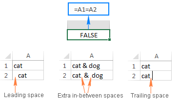
Now that you are fully aware of the problem, it's time to work out a solution. There are several ways to remove spaces from string, and this tutorial will help you choose the technique best suited for your particular task and the data type you are working with.
How to remove blank spaces in Excel - leading, trailing, between words
If your data set contains superfluous spaces, the Excel TRIM function can help you delete them all in one go - leading, trailing and multiple in-between spaces, except for a single space character between words.
A regular TRIM formula is as simple as this:
=TRIM(A2)
Where A2 is the cell you want to delete spaces from.
As shown in the following screenshot, the Excel TRIM formula successfully eliminated all spaces before and after the text as well as consecutive spaces in the middle of a string.
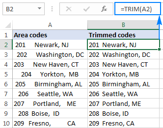
And now, you only need to replace values in the original column with trimmed values. The easiest way to do this is using Paste Special > Values, the detailed instructions can be found here: How to copy values in Excel.
Additionally, you can use the Excel TRIM function to remove leading spaces only, keeping all spaces in the middle of a text string intact. The formula example is here: How to trim leading spaces in Excel (Left Trim).
How to delete line breaks and nonprinting characters
When you import data from external sources, it's not only extra spaces that come along, but also various non-printing characters like carriage return, line feed, vertical or horizontal tab, etc.
The TRIM function can get rid of white spaces, but it cannot eliminate non-printing characters. Technically, Excel TRIM is designed to only delete value 32 in the 7-bit ASCII system, which is the space character.
To remove spaces and non-printing characters in a string, use TRIM in combination with the CLEAN function. As its names suggests, CLEAN is purposed for cleaning data, and it can delete any and all of the first 32 non-printing characters in the 7-bit ASCII set (values 0 through 31) including line break (value 10).
Assuming the data to be cleaned is in cell A2, the formula is as follows:
=TRIM(CLEAN(A2))
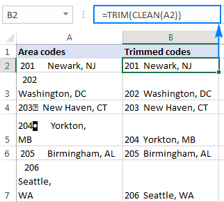
If the Trim/Clean formula joins the contents of multiple lines without spaces, you can fix it by using one of these techniques:
- Utilize the "Replace All" feature of Excel: in the "Find what" box, input a carriage return by pressing the Ctrl+J shortcut; and in the "Replace with" box, type a space. Clicking the Replace All button will swap all line breaks in the selected range for spaces.
- Use the following formula to substitute Carriage Return (value 13) and Line Feed (value 10) characters with spaces:
=SUBSTITUTE(SUBSTITUTE(A2, CHAR(13)," "), CHAR(10), " ")
For more information, please see How to remove carriage returns (line breaks) in Excel.
How to remove non-breaking spaces in Excel
If after using the TRIM & CLEAN formula some stubborn spaces are still there, most likely you copy/pasted the data from somewhere and a few non-breaking spaces sneaked in.
To get rid of nonbreaking spaces (html character ), replace them with regular spaces, and then have the TRIM function remove them:
=TRIM(SUBSTITUTE(A2, CHAR(160), " "))
To better understand the logic, let's break down the formula:
- A non-breaking character has value 160 in the 7-bit ASCII system, so you can define it by using the CHAR(160) formula.
- The SUBSTITUTE function is used to turn non-breaking spaces into regular spaces.
- And finally, you embed the SUBSTITUTE statement into the TRIM function to remove the converted spaces.
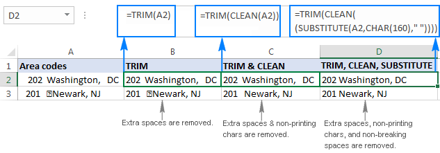
If your worksheet also contains non-printing characters, use the CLEAN function together with TRIM and SUBSTITUTE to get rid of spaces and unwanted symbols in one fell swoop:
=TRIM(CLEAN((SUBSTITUTE(A2,CHAR(160)," "))))
The following screenshot demonstrates the difference:
Tip. If the combination of TRIM, CLEAN, and SUBSTITUTE does not eliminate certain spaces or non-printable characters, those characters likely have ASCII codes outside the standard ranges (0–32 for non-printable characters or 160 for non-breaking spaces). In this case, use the CODE function to determine the character value, and then remove it as shown in this example: Identify and remove specific non-printing characters in Excel.
How to remove all spaces in Excel
In some situations, you may want to remove absolutely all white spaces in a cell, including single spaces between words or numbers. For example, when you have imported a numeric column where spaces are used as thousands separators, which makes it easier to read big numbers, but prevents your formulas from calculating.
To delete all spaces in one go, use SUBSTITUTE as explained in the previous example, with the only difference that you replace the space character returned by CHAR(32) with nothing (""):
=SUBSTITUTE(A2, CHAR(32), "")
Or, you can simply type the space (" ") in the formula, like this:
=SUBSTITUTE(A2," ","")
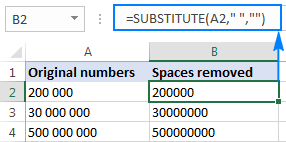
After that, replace formulas with values and your numbers will calculate properly.
How to count spaces in Excel
Before removing spaces from a certain cell, you may be curious to know how many of them are actually there.
To get the total count of spaces in a cell, do the following:
- Calculate the entire string length using the LEN function: LEN(A2)
- Substitute all spaces with nothing: SUBSTITUTE(A2," ","")
- Compute the length of the string without spaces: LEN(SUBSTITUTE(A2," ",""))
- Subtract the "space-free" string length from the total length.
Assuming the original text string is in cell A2, the complete formula goes as follows:
=LEN(A2)-LEN(SUBSTITUTE(A2," ",""))
To find out how many extra spaces are in the cell, get the text length without extra spaces, and then subtract it from the total string length:
=LEN(A2)-LEN(TRIM(A2))
The following screenshot demonstrates both formulas in action:
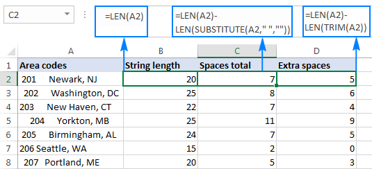
Now that you know how many spaces each cell contains, you can safely delete extra spaces using the TRIM formula.
Formula-free way to remove spaces and clean data
As you already know, many extra spaces and other unwelcome characters can lurk unnoticed in your sheets, especially if you import your data from external sources. You also know how to delete spaces in Excel with a formula. Of course, learning a handful of formulas is a good exercise to sharpen your skills, but it might be time-consuming.
Excel users who value their time and appreciate convenience can take advantage of the Trim Spaces included with our Ultimate Suite for Excel. One of these handy tools allows removing spaces and non-printing characters in a button click.
Once installed, Ultimate Suite adds several useful buttons to your Excel ribbon such as Trim Spaces, Remove Characters, Convert Text, Clear Formatting, and a few more.
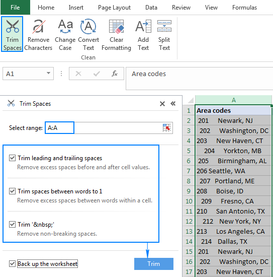
Whenever you want to remove blank spaces in your Excel sheets, perform these 4 quick steps:
- Select the cells (range, entire column or row) where you want to delete extra spaces.
- Click the Trim Spaces button on the Ablebits Data tab.
- Choose one or several options:
- Remove leading and trailing spaces
- Trim extra spaces between words to one
- Delete non-breaking spaces ( )
- Click the Trim button.
Done! All extra spaces are deleted in a single click.
This is how you can quickly remove spaces in Excel cells. If you are curious to explore other capabilities, you are most welcome to download an evaluation version of the Ultimate Suite. I thank you for reading and look forward to seeing you on our blog next week!
 by
by
15 comments
I have a column of data where I would like to remove trailing spaces at the end of text. Some of my text includes two or more spaces within the text that needs to remain intact. So, the TRIM function will not work. There's also no consistency to the trailing spaces either. The text could have any number of trailing spaces.
Here's a couple of examples:
"212Q RML Moultrie GA " <-- this text includes 5 spaces between the "212Q" and "RML" which should not be adjusted. There is also 3 spaces at the end which should be eliminated
"209Q RVI Vidalia GA " <-- this text includes 3 spaces between the "209Q" and "RVI" which should not be adjusted. There is also 10 spaces at the end which should be eliminated
Hello! You can use an Excel formula to remove all extra spaces to the right in a text string. The MID function splits the text string in individual chars. In this example, the string is 100 characters long. Then use the XMATCH function to find the position of the character greater than or equal to "!", starting from the last character. Let's explain that "!" is the first character that is greater than a space. Then we will use the LEFT function to extract the desired number of characters from the text string, not including the spaces at the end.
=LEFT(A1,XMATCH("!",MID(A1,ROW(A1:A100),1),1,-1))
You can also find useful information in this article: Remove leading spaces only (Left Trim).
You can solve the problem without using formulas. We have a tool that can solve your task in a couple of clicks - Trim Spaces tool. It helps you eliminate unnecessary leading and trailing spaces. The tool is included in the Ultimate Suite for Excel and can be used in a free trial to see how it works.
( 12121212) like this situation how to remove space in excel. Thanks
Hi! I hope you have studied the recommendations in the tutorial above. Use the SUBSTITUTE function to replace a space with a blank.
=SUBSTITUTE(A1," ","")
A number has been copied from a table pasted on body of an email. When it is pasted in excel, formula bar reveals white space (more than 1 character long) at the beginning of the no. & at end also. How to eliminate such white space & make the no. a real no. which I can use in calculation?
(My suggestion: a code which will delete all characters excluding nos. 0 to 9)
Hi! If I understand your task correctly, the following tutorial should help: How to remove special (unwanted) characters from string in Excel.
You can also try using regular expressions and the user-defined function RegExpReplace as recommended in these instructions: Regex to remove non-numeric characters. I recommend paying attention to the Regex tool. You can find, extract, compare, delete, or replace strings that match the regular expression pattern you enter. You don't need to install any VBA code.
Hello,
I have an interesting issue which non of the above addresses. I have only one part number in a column which has three trailing spaces which TRIM, CLEAN, and SUBSTITUTE (including CHAR()) does not remove in formula. Here are the steps:
PN = "E30392-I1-UR3-8-W "
1) original cell text from another worksheet (CALL IT SHEET2), referenced to active worksheet (CALL IT SHEET1) using formula
2) when I use =CODE(RIGHT(SHEET2!A1,1)) = 87 which is ASCII code for "W", not unidentifiable space
3) copy then paste as values from formula shows results with "E30392-I1-UR3-8-W" (no space), but I don't want to replace formulas with values
4) tried with TRIM, CLEAN and SUBSTITUTE CHAR(160) to "" but to no avail
5) I don't want to remove inside text spaces, only outside
6) I cannot assume all values in column have same number of trailing spaces (it will chop off good characters in other text if I do)
How to identify ASCII code if it does not see these spaces? How to remove outside spaces without losing inside spaces and good characters in cells?
If I can upload file to you would be better.
Hello! Unfortunately, I can't identify which characters are in your text because I don't have access to your data. Try using our
Ultimate Suite for Excel that you can install in a trial mode and check how it works for free.
Thank you Alexander for quick reply.
My colleague figured out the ASCII code for mysterious spaces are 32. I attempted to use SUBSTITUTE CHAR(32) but still VLOOKUP did not recognize it in lookup table. I forgot to mention about the VLOOKUP. However, after deleting the mysterious spaces from source worksheet (SHEET2), VLOOKUP does find match in table.
I don't have anymore info to give. Hopefully this helps you understand better my situation.
How do I trim ONLY spaces at the end of the cell? There's a double-space at the end of the cell as well as one in the middle of the cell. I don't want to get rid of the one in the middle because subsequent formulas depend on it. How can I only trim the trailing spaces?
Hello!
If there is a double space at the end of each cell, use the MID function to remove the trailing spaces
=MID(A1,1,LEN(A1)-2)
How to remove spaces between two or more than words in excel. for example I want "TheNPLCitation" from "The NPL Citation"
Hello!
Have you carefully studied this article?
You can remove spaces between words using the function SUBSTITUTE
Read the section above carefully How to remove all spaces in Excel
=SUBSTITUTE(A1," ","")
This article saved my life!!! THANK YOU!!! I was struggling finding a way to clean up my google sheets, too many spaces in too many cells and over 5k rows to clean up. This was a godsend.
Hi Bob,
We have a special tool to trim spaces in Google Sheets in all cells at once, feel free to have a look: Remove Excess Spaces