 by
by This article covers the most common data cleaning techniques, from removing extra spaces and duplicates to fixing formatting issues and typos, so you can quickly turn raw data into something accurate and ready to use.
Messy data happens to everyone. One minute you're working with a neat list, and the next you're staring at extra spaces, inconsistent formatting, and mystery characters. The good news? Excel gives you plenty of ways to clean things up, you just need to know where to look 😊
The basics of cleaning Excel data
Data imported from external sources rarely arrives in perfect shape. Before you can analyzing it, a bit of cleanup is usually necessary. Since every dataset comes with its own quirks, there's no one-size-fits-all solution. However, there is a logical approach you can follow to make the process more structured and keep your original data safe.
- Create a backup copy. Before making any changes, copy your dataset to another worksheet or workbook. This gives you a safety net in case something goes wrong.
- Make sure your data is properly structured. Your data should be arranged in a tabular format, where:
- Each column contains one type of data (e.g. names, dates, amounts).
- Each row represents one record.
- There are no completely blank rows or columns in the middle.
- All rows and columns are visible (unhide anything hidden).
- Start with simple fixes. Begin with tasks that don't require changing the structure of your data, such as running spell check or using Find and Replace to correct obvious inconsistencies like "NY" vs "New York".
- Move on to column-based cleaning. Next, handle tasks that require transforming data using formulas. The general steps for manipulating a column are:
- Insert a new column next to the one you want to clean.
- In the top cell of the new column, enter a formula to transform the data (for example, TRIM, CLEAN, or UPPER).
- Copy the formula down by dragging the fill handle down. Or, use a dynamic array formula that spills automatically. Or, convert your data set to an Excel Table that automatically creates calculated columns.
- Convert formulas to values. Select the new column, copy it, then paste it back as values (Paste Special > Values).
- Once you are confident the cleaned data is correct, delete the original column.
Following this process will help you avoid data loss and keep your workflow clear and predictable.
How to clean data in Excel – practical techniques
Below are top ten cleaning data techniques in Excel. They are arranged by frequency of use, with the ones you'll need in most situations placed at the top.
Trim extra spaces
Extra spaces are one of the most common issues when data is copied from an external database, web page, or another application. They can appear at the beginning, end, or between words, and often go unnoticed until something stops working.
To remove leading, trailing, and repeated spaces between words, use the TRIM function. The formula is as simple as this:
=TRIM(A4) Enter the formula in the top cell of a helper column, and then copy it down to clean the rest of the rows.
In Excel 365, you can clean an entire range in one go:
=TRIM(A4:B28) The formula will spill the cleaned results automatically, saving you from filling it down manually.
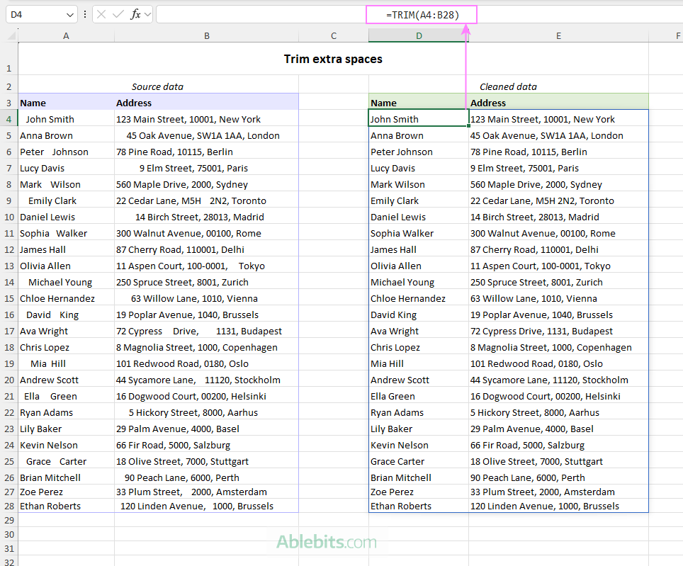
For a deeper dive, see How to remove spaces in Excel.
Note. The TRIM function removes standard spaces but does not handle non-breaking spaces ( ) that often found in web data. To deal with those, combine TRIM with SUBSTITUTE, as explained in How to remove non-breaking spaces in Excel.
Tip. A faster and easier way might be using the Trim Spaces tool included in the Ablebits Ultimate Suite. It can handle everything in one go: extra spaces, non-breaking spaces, and even unwanted line breaks.
Clean non-printable characters
Another frequent problem in Excel, which can break formulas and affect sorting or filtering, is non-printable characters. To get rid of them, use the CLEAN function:
Per-cell formula:
=CLEAN(A4)
Dynamic array formula (for a range):
=CLEAN(A4:B28)
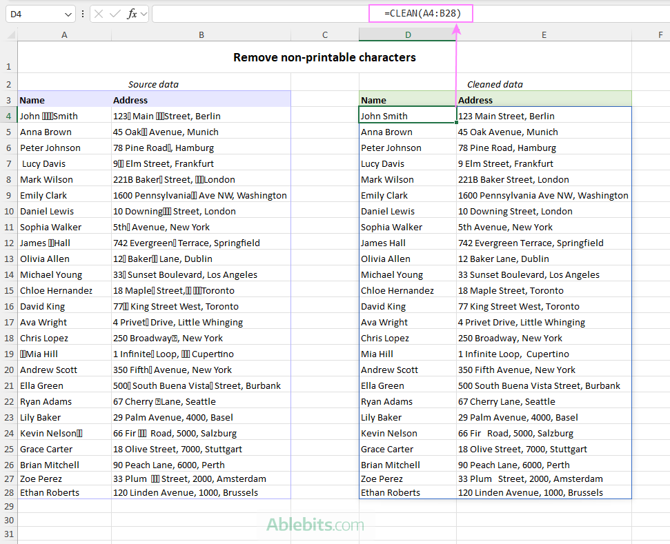
If your dataset contains both non-printable characters and extra spaces, you can eliminate both in one step by combining the TRIM and CLEAN functions:
=TRIM(CLEAN(A4:B28))
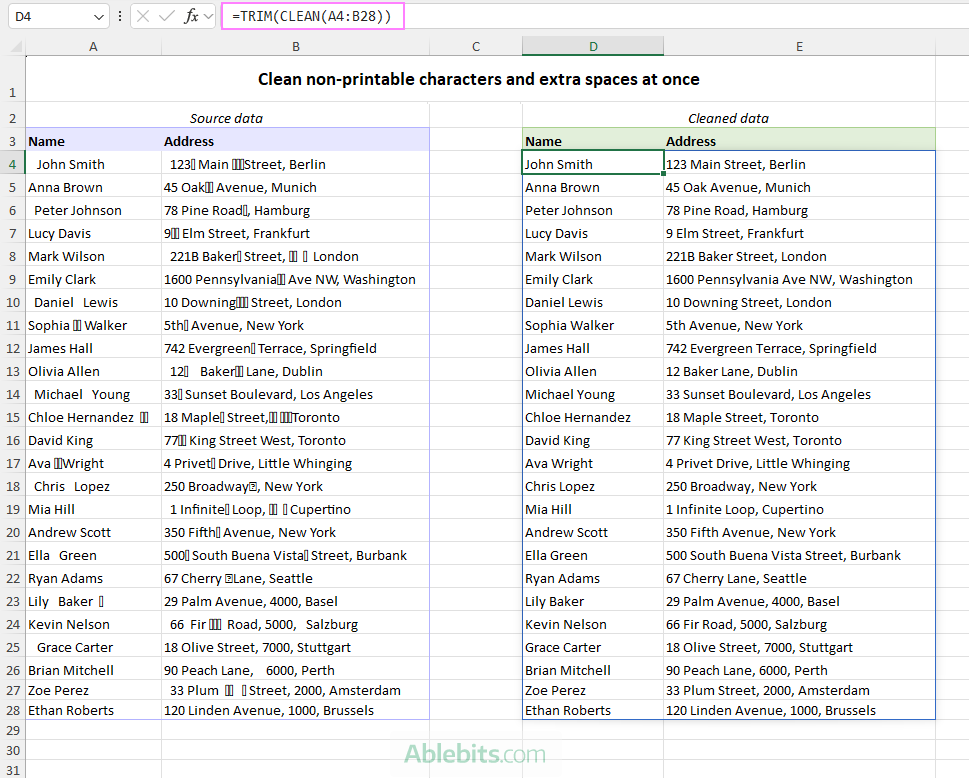
Note. The CLEAN function also removes line breaks. If your data includes multi-line entries that need to be preserved, avoid using this function.
Identify and remove specific non-printing characters
If neither TRIM nor CLEAN was able to eliminate extra spaces or visible "garbage" characters in your sheet, the issue is likely caused by additional non-printable ASCII characters (such as 127, 129, 141, 143, 144, or 157).
In this case, you can use the CODE function to determine the character value, SUBSTITUTE to replace it with a regular space, and TRIM to remove the space.
Step 1. Identify the character
Depending on where the problematic character appears in a cell, use one of these formulas:
Leading space or non-printing character at the beginning of the text string:
CODE(LEFT(cell, 1))
Trailing space or non-printing character at the end of the string:
CODE(RIGHT(cell, 1))
Space or non-printing character in the middle of the string (position n):
CODE(MID(cell, n, 1))
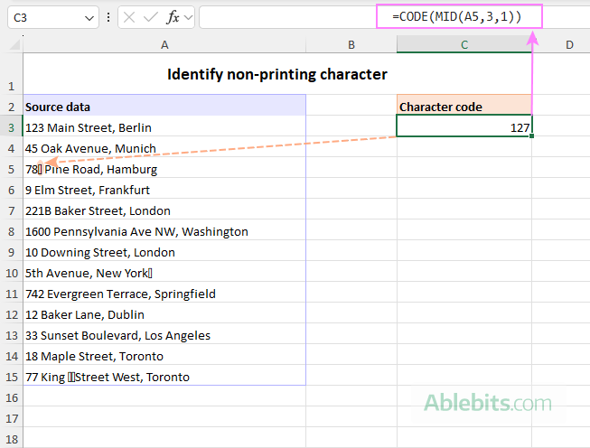
In this example, some unknown character is in the 3rd position of cell A5, so you can find out its value with this formula:
=CODE(MID(A5, 3, 1)) This returns the character code 127 (representing the Delete command), as shown in the screenshot:
Step 2. Remove the character
Once you know the character code, substitute it with a normal space, and trim the result:
=TRIM(SUBSTITUTE(A5, CHAR(127), " "))
If the same character appears in more than one cell, you can clean a whole range using a dynamic array formula like this one:
=TRIM(SUBSTITUTE(A3:A27, CHAR(127), " "))
Remember, dynamic array formulas are only available in Excel 365, 2024 and 2021. In older version, write a formula for the topmost cell and copy it down.
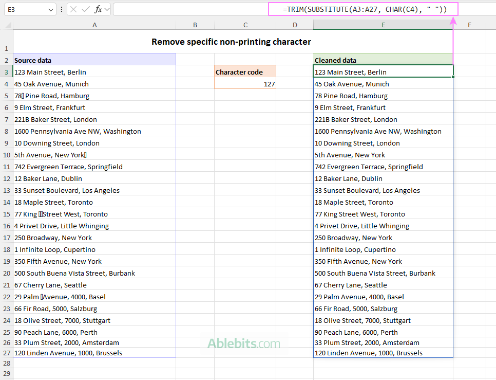
Removing multiple characters at once
If your data contains a few different non-printing symbols, you can nest multiple SUBSTITUTE functions to remove all unwanted character codes at a time.
For example, to get rid of non-printable character 127 and non-breaking spaces (character 160), the formula is:
=TRIM(SUBSTITUTE(SUBSTITUTE(A3:A27, CHAR(127), " "), CHAR(160), " "))
Find and replace certain characters or text
Sometimes your data looks fine at first glance, but a closer look reveals inconsistencies – different spellings, odd symbols, or leftover HTML codes. There are two main methods to fix these issues, depending on the situation.
Method 1: Use Find and Replace
Excel's Find and Replace feature is a quick way to clean up repeated issues in your worksheet. It's especially useful for:
- Standardizing values that appear in multiple variations, for example US, USA, United States.
- Fixing imported characters from web pages, such as – instead of an en dash (–), instead of a space, or ’ instead of an apostrophe (').
For example, here's how we can replace all instances of – with the en dash character:
- Select the range that contains your data.
- Press Ctrl + H to open the Find and Replace dialog.
- In the Find what box, enter the character or text to replace (– in our case).
- In the Replace with box, enter the character to use instead (–).
- Click the Replace All button.
Excel will update all matching entries at once.
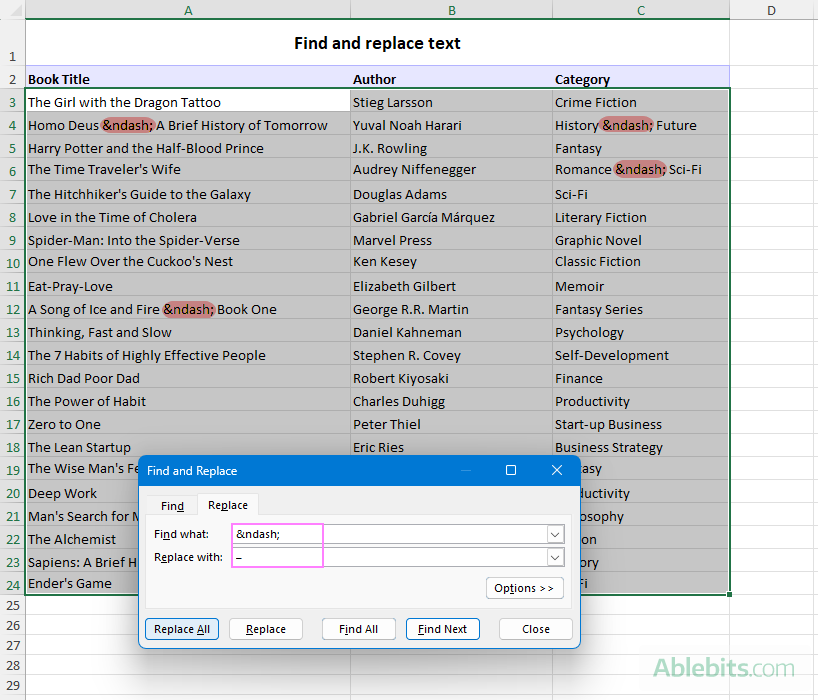
This method works best when you want to replace the same character or text across multiple columns in a single step.
Tip. To remove specific characters or words entirely, leave the Replace with box empty.
Method 2: Replace multiple characters or text using a formula
If your data contains multiple different issues in the same column, using a formula can be faster and more flexible.
For example, suppose column A contains:
- – that should become an en dash (–)
- ’ that should become an apostrophe (')
You can handle both replacements at once with nested SUBSTITUTE functions:
=SUBSTITUTE(SUBSTITUTE(A3:A24, "–", "–"), "’", "'") This formula replaces each unwanted character and returns cleaned results for the entire range.
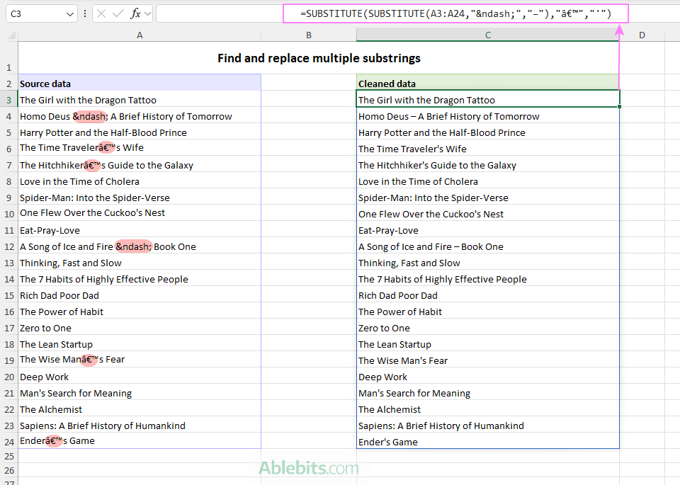
Use this method when:
- You want to perform multiple replacements at once.
- You wish to keep the original data unchanged while working in a helper column.
Eliminate unwanted characters
Sometimes your Excel data contains characters that simply don't belong to it such as extra symbols, formatting leftovers, or artifacts from imported content. To remove unwanted characters, you can use the same two approaches as for replacing text:
- Excel's Find and Replace. Leave the Replace with box empty to delete specific characters.
- Nested SUBSTITUTE formulas. Replace unwanted characters with an empty string.
For example, the formula below removes four different characters (*, ^, %, and ¿) from the range A3:A24. Technically, each character is replaced with a zero-length string (""):
=SUBSTITUTE(SUBSTITUTE(SUBSTITUTE(SUBSTITUTE(A3:A24, "*", ""), "^", ""), "%", ""), "¿", "")
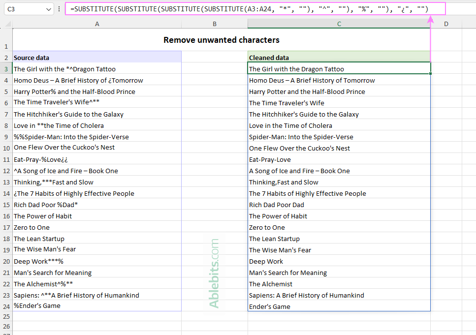
This approach works well when the number of characters to remove is manageable and you know exactly which ones need to be deleted.
If you have many different characters that you want to get rid of, these basic methods may not be enough. For bulk replacement, consider more advanced options like LAMBDA, VBA or Ablebits' Remove Characters tool.
For step-by-step guidance, see How to remove unwanted characters in Excel.
Remove duplicates
Duplicate values are another frequent source of errors in Excel sheets and often one of the trickiest to deal with. That's because "duplicates" can mean different things depending on your data and goal.
Here are the main scenarios:
- Duplicate cells. You may want to remove all repeated values or keep only the first occurrence.
- Duplicate rows. These can be exact matches across all columns or partial matches based on one or more key columns.
- Duplicates within a cell. A single cell may contain repeated words or text strings.
Because of these variations, the right solution depends on how you define a duplicate in your dataset. Based on your understanding, choose an appropriate method:
- Find and remove duplicate cells – with or without keeping the first occurrence.
- Remove duplicate rows – based on matching values in one or more columns
- Remove duplicates in Excel cell – remove repeated words or text within a single cell.
- How to find duplicates in Excel – identify them before removing by highlighting, counting, or filtering.
Alternative tool: Duplicate Remover for Excel by Ablebits is an all-in-one tool that can find, highlight, remove, or copy duplicate or unique values in one or multiple columns.
Fix inconsistent text case
Text in Excel is not always entered consistently. In the same dataset, you might see some values in uppercase, others in lowercase, and some in a random mix that looks like caps lock had a personality 😊
To standardize letter case, Excel provides three simple functions:
- UPPER – converts text to uppercase.
- LOWER – converts text to lowercase.
- PROPER – capitalizes the first letter of each word.
For example, to convert all text in the range A3:B23 to proper case, use this formula:
=PROPER(A3:B23) This comes in handy for cleaning names, titles, addresses, and other text that should follow a consistent style.
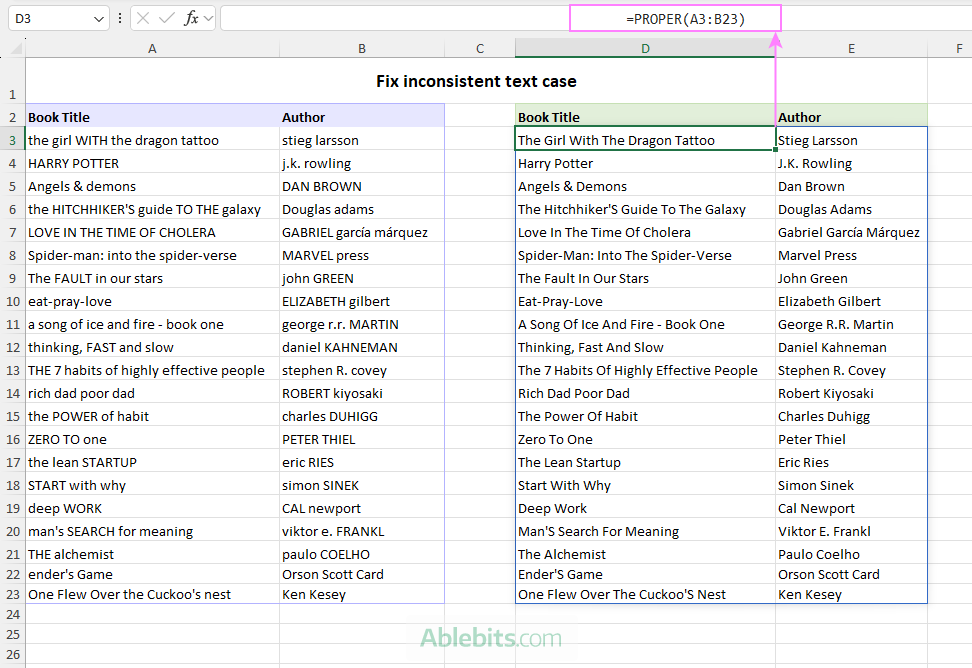
Note. Be careful when using the PROPER function with possessive forms. It treats the suffix 's as a separate word and capitalizes it as 'S.
Besides the built-in case functions, you can also use these alternatives:
- Convert text case with VBA macro – 3 code samples to convert text to uppercase, lowercase and proper / title case.
- Cell Cleaner add-in – a dedicated tool in the Ablebits Ultimate Suite that lets you change text case without formulas.
Convert numbers stored as text to numbers
Numbers stored as text are a widespread issue in Excel that can quietly break calculations and charts. They may look like numbers, but Excel treats them as text, therefore formulas won't work as expected.
The quickest fix is to use the built-in option: click the warning icon in the affected cell and choose Convert to Number.
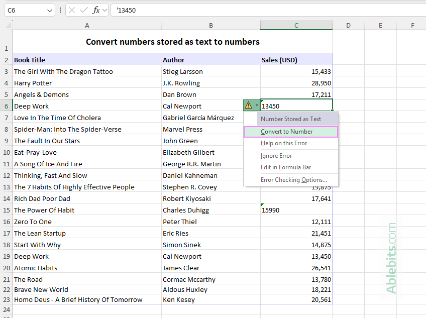
If you are dealing with multiple cells, try one of these formulas:
Multiply by 1:
=C3:C23*1
Use the VALUE function:
=VALUE(C3:C23)
Both methods force Excel to recognize the values as numbers.
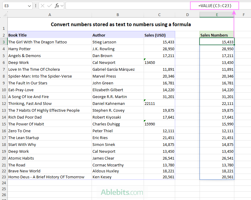
For more details on how to identify numbers stored as text and fix them in different scenarios, see How to convert text to number in Excel.
Handle blank cells, rows and columns
Blank cells are not always a problem in Excel worksheets. In some datasets, they are perfectly fine and simply mean that the data is not available or not applicable. In other cases, blanks may indicate missing or incomplete information that needs attention.
Because of this, there isn't a single "right" way to deal with blanks in Excel, as different situations call for different solutions.
Here are the most common ways to handle blank cells in Excel:
Delete blank cells
If blanks are not needed, you can remove them. However, be careful – deleting empty cells incorrectly can shift data and break your dataset. Avoid deleting entire rows or columns if they contain valid data alongside blanks.
The below articles explain how to delete blanks safely:
Highlight blanks
Before deleting anything, it's often a good idea to identify blank cells first. This helps you understand how widespread the issue is and reduces the risk of removing important data by mistake.
You can highlight blanks using filtering, Go To Special, conditional formatting, or VBA. All of these methods are explained in detail in How to select and highlight blank cells in Excel.
Fill blank cells
In some situations, filling gaps in your data is a better option than deleting empty cells, particularly when you want to preserve the structure of your dataset. The options are:
- Replacing blanks with 0 or a custom value like "N/A".
- Filling cells with values from above or below.
For a more in-depth explanation, see How to fill empty cells with 0 or value above/below.
Standardize date and time formats
Dates and times can appear in many different formats depending on the source of your data. For example, you might see 01/05/2024, May 1, 2024, and 2024-05-01 all in the same column. While they may represent the same value, inconsistent formatting can make your data harder to read and work with.
To quickly apply a consistent format, use the Number Format drop-down on the Home tab:
- Select your date or time range.
- Choose Short Date, Long Date, or Time.
This will update all selected values to your system's default date or default time format.
Apply a custom date / time format
If you need more control over how dates or times are displayed, use the Format Cells dialog:
- Select the cells with dates or times you want to format.
- Press Ctrl + 1 to open the Format Cells dialog.
- Go to the Number tab and choose Date or Time.
- Under Type, select the format you prefer.
- Click OK to apply the changes.
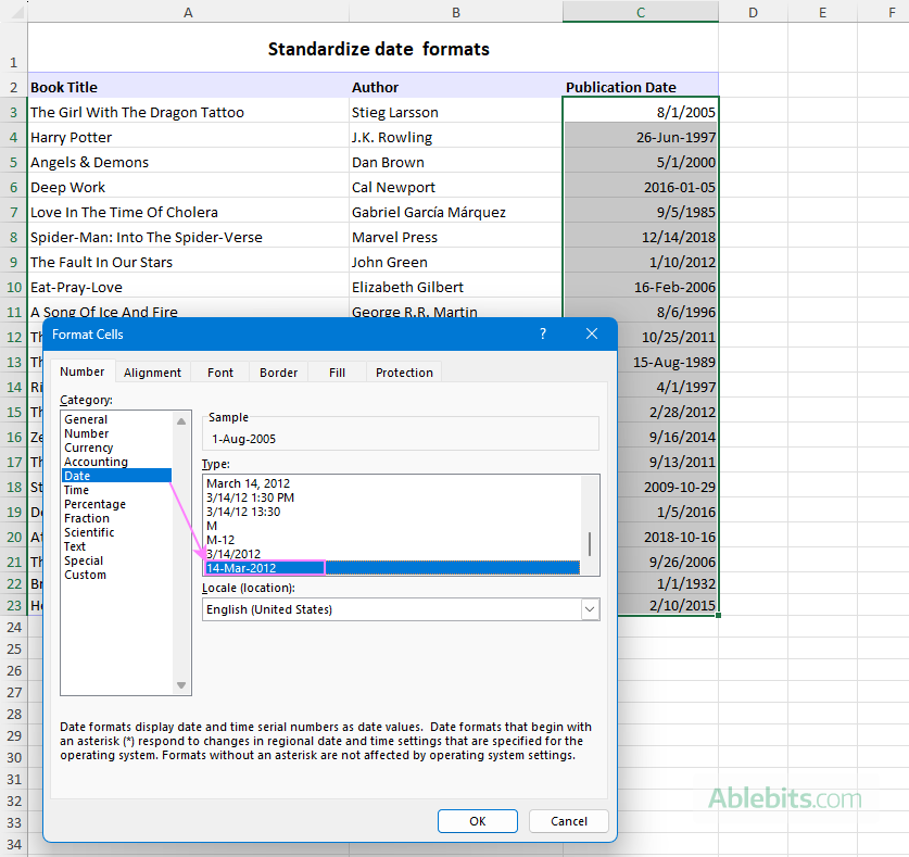
Note. If the format does not change, your dates are likely stored as text. In that case, convert them to real dates first before applying formatting.
For a detailed walkthrough, see:
Check for misspelled words and typos
Misspelled words and typos are easy to overlook, especially in large datasets. Even small inconsistencies can affect searches, filtering, and overall data quality.
There are three main ways to check and correct spelling in Excel:
Spell Checker
You can use Excel's built-in spell-checking tool to:
- Find misspelled words in a selected range, multiple sheets, or the entire workbook.
- Identify inconsistently used terms (e.g. product or company names) by adding them to a custom dictionary.
- Check text returned by formulas. By default, Excel does not check text in formula results. But if you enter edit mode in a cell and then run spell check, it will evaluate custom text used in a formula.
Macros
You can automate spell checking across the active sheet or the entire workbook. If needed, VBA macros can also highlight misspelled words by changing the cell background color.
Fuzzy Duplicate Finder
Fuzzy Duplicate Finder is a specialized add-in that finds similar entries with small differences (1 to 10 character variations), including missing, extra, or mistyped characters.
To explore these approaches in detail, see How to spell check in Excel.
How to clean Excel data with Copilot
If Excel Copilot is included in your Microsoft 365 subscription, it can help you detect some typical issues and suggest fixes. You can then review and apply the changes directly from the Copilot pane.
What kind of data can Copilot clean up?
Copilot is designed to handle the most common data quality problems, such as:
- Spacing issues. Removes extra spaces at the beginning, end, or between words.
- Inconsistent capitalization. For example, it can standardize entries like john smith, JOHN SMITH, and John Smith.
- Inconsistent formatting. For example, it can align variations like 1-2 days, 1 – 2 days, and 1 - 2 days.
Note. Copilot does not handle all types of data problems. For example, it may not remove non-printing and other "garbage" characters or fix inconsistent date formats.
How to clean your data with Copilot
Using Copilot is straightforward once your data is properly prepared.
- Format your data for Copilot. Ensure your data is in a supported format, such as an Excel table or a structured range (unique column headers, no subtotals, no blank rows or columns, no merged cells).
- Run the Clean Data tool. On the Data tab, in the Data Tools group, click Clean Data.
- Review suggested fixes. Copilot scans your dataset and highlights issues such as spacing, capitalization, and formatting inconsistencies in its pane.
- Apply or ignore changes. Review each suggestion and choose Apply to update your data or Ignore to keep the original values.
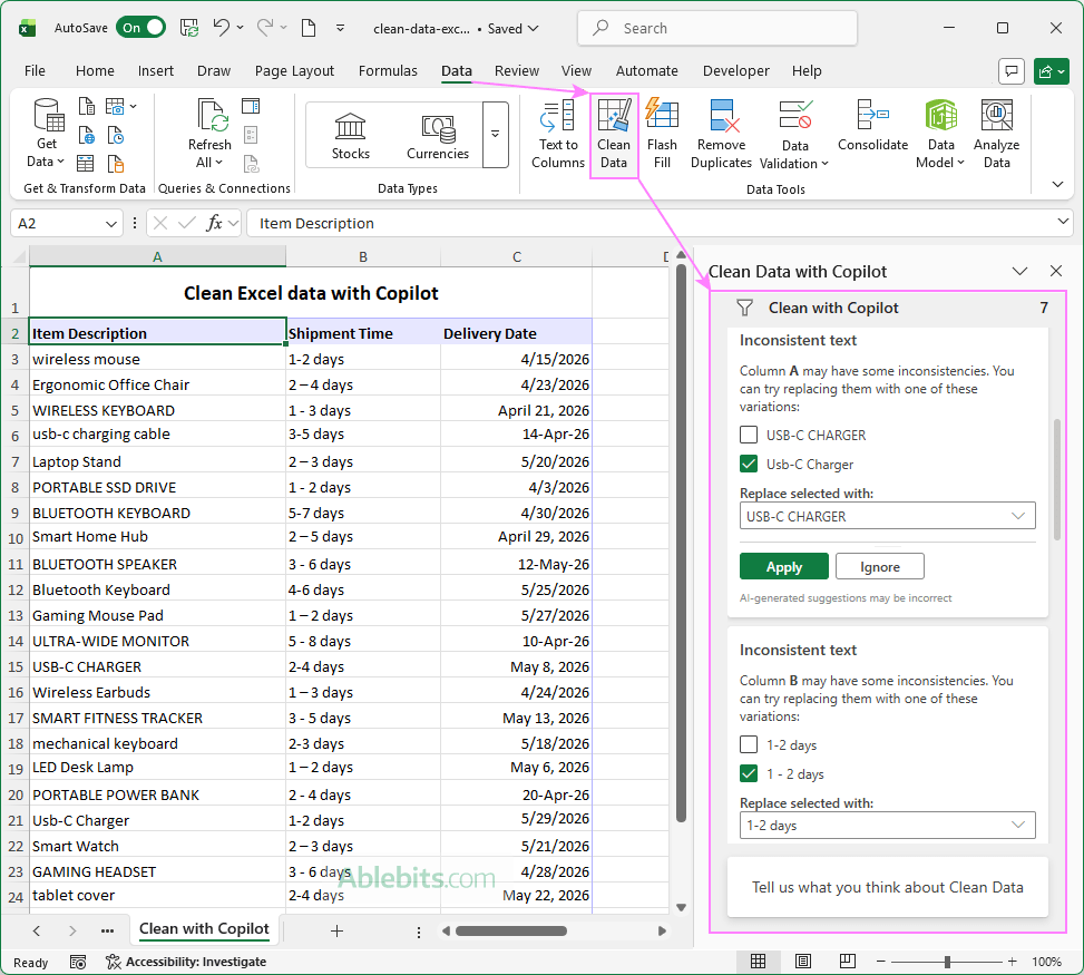
Copilot is especially helpful for quick cleanups, while more complex issues may still require formulas or manual adjustments.
These methods cover the essentials of cleaning Excel data. Once you've used them a few times, you'll notice patterns and fix issues much faster. Below, you will find a few additional techniques that can help you handle more specific situations.
Practice workbook for download
How to clean data in Excel - examples (.xlsx file)