This tutorial explains how to calculate interest rate on recurring deposit in Excel by using the RATE function.
Financial decisions are an important element of business strategy and planning. In everyday life, we also have quite a lot of financial decisions to make. For instance, you are going to apply for a loan to buy a new car. It will surely be helpful to know exactly what interest rate you will have to pay to your bank. For such scenarios, Excel provides the RATE function that is specially designed for calculating interest rate for a specific period.
Excel RATE function
RATE is an Excel financial function that finds an interest rate per a given period of an annuity. The function calculates by iteration and can have no or more than one solution.
The function is available in all versions Excel 365 - 2007.
The syntax is as follows:
Where:
- Nper (required) - the total number of payment periods such as years, months, quarters, etc.
- Pmt (required) - the fixed payment amount per period that cannot be changed over the life of the annuity. Usually, it includes principal and interest, but no taxes.
- Pv (required) - the present value, i.e. the current value of the loan or investment.
- Fv (optional) - the future value, i.e. the cash balance you wish to have after the last payment. If omitted, it defaults to 0.
- Type (optional) - indicates when the payments are made:
- 0 or omitted (default) - payment is due at the end of the period
- 1 - payment is due at the beginning of the period
- Guess (optional) - your assumption for what the rate might be. If omitted, it defaults to 10%.
7 things you should know about Excel RATE function
To efficiently use RATE formulas in your worksheets, please pay attention to these usage notes:
- The RATE function calculates through trial and error. If it fails to converge to a solution after 20 iterations, a #NUM! error is returned.
- By default, an interest rate is calculated per payment period. But you can derive an annual interest rate by multiplication as shown in this example.
- Use positive numbers to represent cash that you receive (inflows) and negative numbers to represent cash that you pay out (outflows).
- Although the RATE syntax describes pv as the required argument, it can actually be omitted if you include the fv argument. Such syntax is typically used for calculating interest rate on a saving account.
- The guess argument can be omitted in most cases because it's just a starting value for an iterative procedure.
- When calculating RATE for different periods, make sure you are consistent with the values supplied for nper and guess. For example, if you are to make annual payments on a 3-year loan at 8% annual interest, use 3 for nper and 8% for guess. If you are going to make monthly payments on the same loan, then use 3*12 for nper and 8%/12 for guess.
- Use RATE when all cash flows are the same and occur through equal intervals of time. If cash flow amounts change but occur at regular intervals, then calculate internal rate of return using the IRR function. When varying cash flows occur at irregular intervals, use the XIRR function to get internal rate of return for non-periodic cash flows.
Basic RATE formula in Excel
In this example, we'll look at how to make a RATE formula in its simplest form to calculate interest rate in Excel.
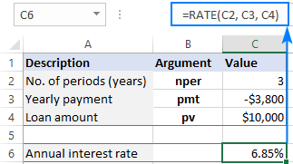
Let's say you've borrowed $10,000 that should be paid in full over the next three years. You are planning to pay 3 yearly installments of $3,800 each. What will the annual interest rate be?
To find it out, we define the following arguments for the Excel RATE function:
- Nper in C2 (number of payments): 3
- Pmt in C3 (payment amount): -3,800
- Pv in C4 (loan amount): 10,000
Please notice that we specify annual payment (pmt) as a negative number because it's outgoing cash.
It's assumed that the payment is to be made at the end of each year, so we can omit the [type] argument or set it to the default value (0). The other two optional arguments [fv] and [guess] are also omitted.
As the result, we get this simple formula:
=RATE(C2, C3, C4)
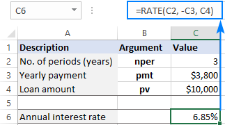
If it is required that the payment be entered as a positive number, then put the minus sign before the pmt argument directly in the formula:
=RATE(C2, -C3, C4)
How to calculate interest rate in Excel - formula examples
Now that you know the essentials of using RATE in Excel, let's explore a couple of specific use cases.
How to calculate monthly interest rate on a loan
Since most installment loans are paid monthly, it may be helpful to know a monthly interest rate, right? For this, you just need to supply an appropriate number of payment periods to the RATE function.
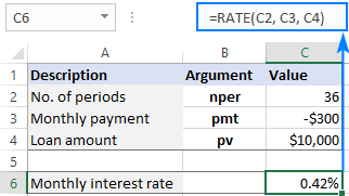
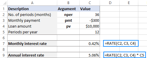
Suppose the loan is to be paid over 3 years in monthly installments. To get the total number of payments, we multiply 3 years by 12 months (3*12=36).
The other parameters are shown below:
- Nper in C2 (number of periods): 36
- Pmt in C3 (monthly payment): -300
- Pv in C4 (loan amount): 10,000
Assuming the payment is due at the end of each month, you can find a monthly interest rate by using the already familiar formula:
=RATE(C2, C3, C4)
Compared to the previous example, the difference is only in the values used for the RATE arguments. Because the function returns an interest rate is for a given payment period, we get a monthly interest rate as the result:
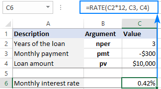
If your source data includes the number of years over which the loan must be repaid, you can do the multiplication inside the nper argument:
=RATE(C2*12, C3, C4)
How to calculate annual interest rate in Excel
Taking our example a little further, how do you find annual interest rate for monthly payments? Simply by multiplying the RATE result by the number of periods per year, which is 12 in our case:
=RATE(C2, C3, C4) * 12
The below screenshot lets you compare the monthly interest rate in C7 and the annual interest rate in C9:
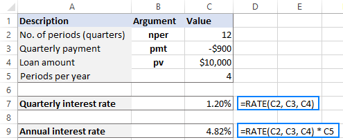
What if the payments are to be made at the end of each quarter?
First, you convert the total number of periods into quarterly:
Nper: 3 (years) * 4 (quarters per year) = 12
Then, use the RATE function to calculate the quarterly interest rate (C7):
=RATE(C2, C3, C4)
And multiply the result by 4 to get the annual interest rate (C9):
=RATE(C2, C3, C4) * 4
How to find interest rate on saving account
In the above examples, we were dealing with loans and calculated the interest rate based on three primary components: loan term, payment amount per period, and loan amount.
Another common scenario is finding an interest rate on a series of periodic cash flows where we know the future value, not the present value.
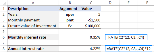
As an example, let's calculate an interest rate required to save up $100,000 in 5 years, provided you make the $1,500 payment at the end of each month with zero initial investment.
To have it done, we define the following variables:
- Nper in C2 (total number of payments): 5*12
- Pmt in C3 (monthly payment): -1,500
- Fv in C4 (desired future value): 100,000
To calculate monthly interest rate, the formula in C6 is:
=RATE(C2*12, C3, ,C4)
Please note that C2 contains the number of years. To get the total number of payment periods, we multiply it by 12.
To get annual interest rate, we multiply the monthly rate by 12. So, the formula in C8 is:
=RATE(C2*12, C3, ,C4) * 12
How to find compound annual growth rate on investment
The RATE function in Excel can also be used for calculating the compound annual growth rate (CAGR) on an investment over a given period of time.
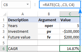
Supposing you want to invest $100,000 for 5 years and receive $200,000 in the end. How will your investment grow in terms of CAGR? To find that out, you set up the following arguments for the RATE function:
- Nper (C2): 5
- Pv (C3): -100,000
- Fv (C4): 200,000
Please pay attention that the pmt argument is not used in this case, so we leave it blank in the formula:
=RATE(C2, ,C3, C4)
As the result, the Excel RATE function tells us that our investment has earned the 14.87% compound annual growth rate over 5 years.
Create interest rate calculator in Excel
As you may have noticed, the previous examples focused on solving specific tasks. This time, our goal is to create a universal interest rate calculator for annuity, which is a series of equal payments made at regular intervals.
Since we will be using an Excel RATE formula in its full form, we need to provide cells for all the arguments, including the optional ones:
- Total number of payments (nper) - C2
- Payment amount (pmt) - C3
- Annuity present value (pv) - C4
- Annuity future value (fv) - C5
- Annuity type (type) - C6
- Estimated interest rate (guess) - C7
- Number of periods per year - C8
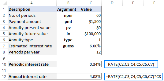
To test our calculator in practice, let's try to find a monthly and annual interest on a saving account that will ensure $100,000 at the end of 5 years with a monthly payment of $1,500 made at the beginning of each period.
We input the variables in corresponding cells like shown in the image below, and enter the following formulas:
In C10, return a periodic interest rate:
=RATE(C2, C3, C4, C5, C6, C7)
In C11, output an annual interest rate:
=RATE(C2, C3, C4, C5, C6, C7) * C8
For our sample data, the results look as follows:
Please note that:
- For nper, we input 60 (5 years * 12 months = 60 payment periods).
- For type, we input 1 (payment is due at the beginning of the period). To prevent mistakes, it makes sense to create a drop-down list in C6 to only allow 0 and 1 values for the type argument.
- If pv is 0 or not defined (like in this example), be sure to specify the fv argument.
Excel RATE function not working
The more complex the function, the greater chance of an error. The RATE syntax is quite simple, but it still leaves room for mistakes, especially if you have little experience with Excel financial functions. Below, we will point out a few common errors and how to fix them.
#NUM! error
Reason: occurs when the RATE function fails to find a solution.
Most often, this happens because positive numbers are used to represent outgoing cash flows. Please remember to put the minus sign before any amount that is paid out:

In some cases, you may need to help the RATE function to converge to a solution by providing an initial guess:

When calculating an interest rate with an undefined or zero present value (pv), be certain to specify the future value (fv):

For more details, see Excel #NUM error: causes and fixes.
#VALUE! error
Reason: occurs when one or more arguments are non-numeric.
To fix the error, double check the values used for the RATE arguments and make sure your numbers are not formatted as text.
RATE function returns incorrect result
Symptom: The result of your RATE formula is a negative percentage, or much lower or higher than expected.
Reason: When calculating monthly or quarterly payments, you forgot to convert the number of years to the total number of payment periods. Or a periodic interest rate is not converted to an annual interest rate.
To resolve this issue, use the following calculations to express the nper argument in appropriate units:
Monthly payments: nper = years * 12
Quarterly payments: nper = years * 4
To get an annual interest rate, multiply a periodic interest rate returned by the function by the number of periods per year.
Monthly payments: annual interest rate = RATE() * 12
Quarterly payments: annual interest rate = RATE() * 4

RATE formula returns zero percentage
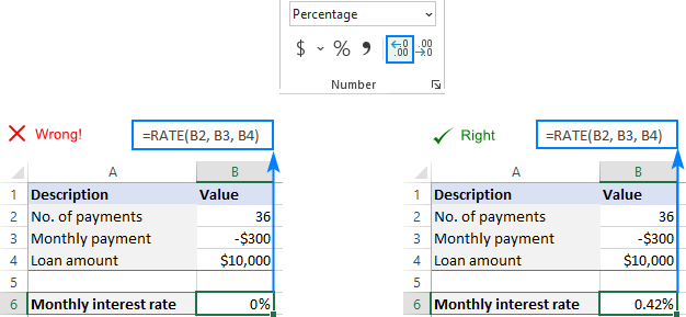
Symptom: The result of the formula appears as zero percentage with no decimal places (0%).
Reason: The calculated interest rate is less than 1%. Because the formula cell is formatted to show no decimal places, the displayed value is "rounded" to zero.
To solve this problem, simply apply the Percentage format with two or more decimal places to the cell containing your formula.
That's how to use RATE function in Excel to calculate interest rate. I thank you for reading and hope to see you on our blog next week!
Practice workbook for download
Examples of RATE formula in Excel (.xlsx file)
 by
by