This short tutorial explains what AutoSum is and shows the most efficient ways to use AutoSum in Excel. You will see how to automatically sum columns or rows with the Sum shortcut, sum only visible cells, total a selected range vertically and horizontally in one go, and learn the most common reason for Excel AutoSum not working.
Did you know that Excel SUM is the function that people read about most? To make sure, just check out Microsoft's list of 10 most popular Excel functions. No wonder they decided to add a special button to the Excel ribbon that inserts the SUM function automatically. So, if you wanted to know "What is AutoSum in Excel?" you already got the answer :)
In essence, Excel AutoSum automatically enters a formula to sum numbers in your worksheet. For more details, check out the following sections of this tutorial.
Where is the AutoSum button in Excel?
The AutoSum button is available in 2 locations on the Excel ribbon.
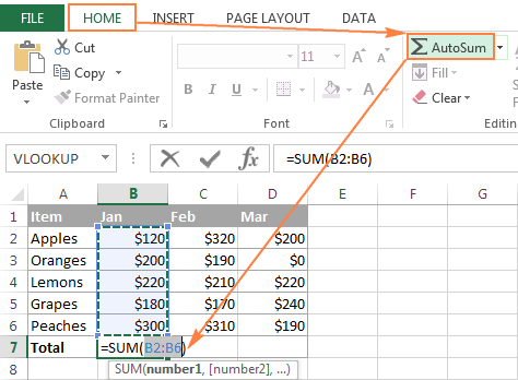
- Home tab > Editing group > AutoSum:

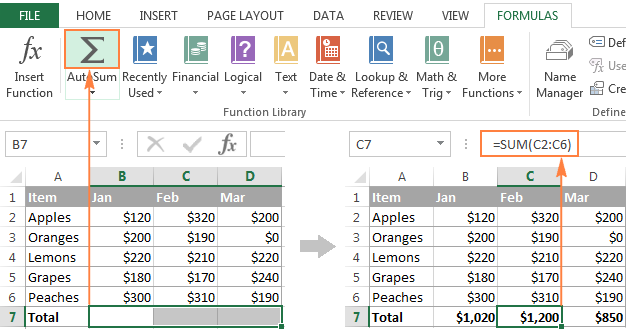
- Formulas tab > Function Library group > AutoSum:

How to AutoSum in Excel
Whenever you need to sum a single range of cells, whether a column, row or several adjacent columns or rows, you can have Excel AutoSum to automatically make an appropriate SUM formula for you.
To use AutoSum in Excel, just follow these 3 easy steps:
- Select a cell next to the numbers you want to sum:
- To sum a column, select the cell immediately below the last value in the column.
- To sum a row, select the cell to the right of the last number in the row.

- Click the AutoSum button on either the Home or Formulas tab.
A Sum formula appears in the selected cell, and a range of cells you're adding gets highlighted (B2:B6 in this example):

In most cases, Excel selects the correct range to total. In a rare case when a wrong range is selected, you can correct it manually by typing the desired range in the formula or by dragging the cursor through the cells you want to sum.
Tip. To sum multiple columns or rows at a time, select several cells at the bottom or to the right of your table, respectively, and then click the AutoSum button. For more details, please see How to use AutoSum on more than one cell at a time.
- Press the Enter key to complete the formula.
Now, you can see the calculated total in the cell, and the SUM formula in the formula bar:

Shortcut for Sum in Excel
If you one of those Excel users that prefer working with the keyboard rather than the mouse, you can use the following Excel AutoSum keyboard shortcut to total cells:

Pressing the Equal Sign key while holding the Alt key inserts a Sum formula in a selected cells(s) exactly like pressing the AutoSum button on the ribbon does, and then you hit the Enter key to complete the formula.
How to use AutoSum with other functions
Apart from adding cells, you can use Excel's AutoSum button to insert other functions, such as:
- AVERAGE - to return the average (arithmetic mean) of numbers.
- COUNT - to count cells with numbers.
- MAX - to get the largest value.
- MIN - to get the smallest value.
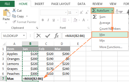
All you need to do is select a cell where you want to insert a formula, click the AutoSum drop-down arrow, and choose the desired function from the list.
For example, this is how you can get the largest number in column B:

If you select More Functions from the AutoSum drop-down list, Microsoft Excel will open the Insert Function dialog box, like it does when you click the Insert Function button on the Formulas tab, or the fx button on the Formula bar.
How to AutoSum only visible (filtered) cells in Excel
You already know how to use AutoSum in Excel to total a column or row. But did you know that you can use it to sum only visible cells in a filtered list?
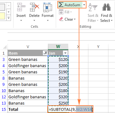
If your data in organized in an Excel table (which can be easily done by pressing Ctrl + T shortcut), clicking the AutoSum button inserts the SUBTOTAL function that adds only visible cells.
In case you've filtered your data by applying one of the Filtering options, clicking the AutoSum button also inserts a SUBTOTAL formula rather than SUM, as shown in the below screenshot:

For more detailed explanation of the SUBTOTAL function arguments, please see How to sum filtered cells in Excel.
Excel AutoSum tips
How that you know how to use AutoSum in Excel to automatically add cells, you may want to learn a couple of time-saving tricks that could make your work even more efficient.
How to use AutoSum on more than one cell at a time
If you want to sum values in several columns or rows, select all the cells where you want to insert the Sum formula, and then click the AutoSum button on the ribbon or press the Excel Sum shortcut.
For example, you can select cells A10, B10 and C10, click AutoSum, and total 3 columns at once. As shown in the below screenshot, the values in each of the 3 columns are summed individually:

How to sum selected cells vertically and horizontally
To total only certain cells in a column, select those cells and click the AutoSum button. This will total the selected cells vertically column-by-column, and place the SUM formula(s) below the selection:

If you want to sum cells row-by-row, select the cells you want to total and one empty column to the right. Excel will sum the selected cells horizontally and insert the SUM formulas to the empty column included in the selection:

To sum cells column-by-column and row-by-row, select the cells you want to add, plus one empty row below and one empty column to the right, and Excel will total the selected cells vertically and horizontally:

How to copy an AutoSum formula to other cells
Once AutoSum has added a SUM (or other) function in the selected cell, the inserted formula behaves like a normal Excel formula. Consequently, you can copy that formula to other cells in the usual way, for example by dragging the fill handle. For more information, please see How to copy a formula in Excel.
Just keep in mind that Excel's AutoSum uses relative cell references (without $) that adjust to the new formula location based on the relative position of rows and columns.
For example, you can have AutoSum to insert the following formula in cell A10 to total the values in column A: =SUM(A1:A9). And when you copy that formula to cell B10, it will turn into =SUM(B1:B9) and total the numbers in column B.
In most cases, it is exactly what you need. But if you want to copy the formula to another cell without changing the cell references, you'd need to fix the references by adding the $ sign. Please see Why use $ in Excel formulas for full details.
Excel AutoSum not working
The most common reason for AutoSum not working in Excel is numbers formatted as text. At first sight, those values may look like normal numbers, but Excel regards them as text strings and does not include in calculations.
The most obvious indicators of numbers formatted as text are their default left alignment and little green triangles in top-left corner of the cells. To fix such text-numbers, select all problematic cells, click the warning sign, and then click Convert to Number.

Numbers can become formatted as text because of various reasons, such as importing a dataset from an external source, or enclosing numeric values in double quotes in your Excel formulas. If the latter, neither green triangles nor the warning sign will appear in cells, because Excel assumes you want to output a text string on purpose.
For example, the following IF formula appears to be working fine:
=IF(A1="OK", "1", "0")
But the returned 1's and 0's are text values, not numbers! And therefore, when you try to do AutoSum on cells containing such formulas, you will always get '0' as the result.
As soon as you remove "" surrounding 1 and 0 in the above formula, Excel AutoSum will treat the outputs as numbers and they will be added up correctly.
If text-numbers are not the case, you can learn about other possible reasons in this tutorial: Excel SUM not working - reasons and solutions.
Well, this is how you do AutoSum in Excel. And if someone ever asks you "What does AutoSum do?", you can refer them to this tutorial :)
Apart from the common SUM function, did you know that Excel has a couple of other functions to conditionally sum cells? If you are curious to learn them, check out the resources at the end of this page. I thank you for reading and hope to see you on our blog next week!
 by
by
34 comments
When using Autosum Feature and you have plus and minus amounts will it pick both up or will it just add up all the amounts and i need to filter the minus amounts?
Hi! You can check this yourself with a simple example. All numbers are summed by the Autosum Feature. If you want to find the sum of only positive numbers in a range, use the SUMIF function. For example:
=SUMIF(A1:A5,">0",A1:A5)
Hi,
From an electric grid provider I have extracted my data to Excel. The data comes in general format and the "numbers" are to the left in the field. If I make a manual formula with field1 + field 2 , I get the correct numbers calculated.
But when I use Autosum , the values are not calculated. I have tried to change the format from general to numeric but it does not help.
If I type manually the value in the field, it calculates the value and the numbers move from the left side of the field to the right side of the field.
Any help much appreciated. Per
Hi! You cannot perform Autosum because your numbers are written as text. I recommend using these guidelines: Excel: convert text to number with formula and other ways.
Hello, I am trying to manually add a number into column A (hours I worked) and have it automatically calculate the difference from a set number (hours currently available) into column B. for each day of the month. I can't figure out how to get it to automatically fill in Column B after I put in the number for Column A. Any help would be greatly appreciated. I have to do this for 30 employees every month and it is so time consuming to manually put in A and B columns for everyone.
Hi!
Write the formula in cell B1. =100-A1
100 is the set number. If the data is down rows, then copy this formula down column B.
I want to add a range of numbers on a column that may change it's length with each use. Add to that I want to do 25 calculations covering the equal parts of the column. So specifically calculating the sum of the first 4% of rows, then the next 4% of rows, etc.
Example A
A column 8,000 rows deep. I want the first calculation to sum rows 1-320 "=Sum(a1:a320)" & "=Sum(a321:a640)" etc
Example B
Next time I use the sheet the column is 12,100 rows deep. I want that formula to automatically change to "=Sum(a1:a484)" & "=Sum(a485:a968)" etc
Right now I have to change the sum range every time I calculate new data. So you can see my interest in a way to have the range automatically change depending on the length of the column.
Thanks for any response, in advance.
Hello!
Create a dynamic named range in column A. For this, you can use the formula:
=OFFSET($A$1, 0, 0, COUNTA($A:$A), 1)
If the name of this dynamic range is "test1", then the SUM formula using the INDIRECT function could be:
=SUM(INDIRECT("A1:A"&ROUND(COUNTA(test1)*0.04,0)))
I hope this will help
Thank you, Alexander.
I went through a little trial and error and needed some creative data filtering but your solution seems to have worked well.
What formula would i use to sum the numbers giving to A1 in each interval and which would display on B1.
For example :1st time i enter 15 in A1 so B1 displays 15
2nd time i enter 20 in A1 so B1 must display "35"
3rd time when A1 = 5 then B1 must be "40"
Hi!
If I understood correctly, what you want to do is impossible. The cell can only store the last value.
HOW TO MAKE A CALCULATION FROM THREE DEFFERENT COLUMN ?
FOR Example: firts colum is 1box equivalent of 60pcs,second column 1packet equivalent of 30pcs then third colomn by pcs.then total of all column.
Thanks for your responce.
Hello!
What formula you used and what problem or error occurred?
You can learn more about SUM function in Excel in this article on our blog.
how to calculate the percentage of gst for examplse 347+18%
pls reply to this mail id
Hello!
Please have a look at this article — How to calculate percentage in Excel – percent formula examples
Hi
How the total production figure in A2 will be changed automatically if I change A1 value.
Let's say yesterday A2 was 1500 and today A1 entered as 100. So how A2 will be 1600.
Hello!
Read how to calculate running total
I hope it’ll be helpful.
How do I autosum only numbers in bold in a column?
Hello, Scott,
Unfortunately, it is not possible to sum only the bold cells using the standard Excel functions. Most likely you need a special macro. I am really sorry we can’t help you with this.
You may try to find the solution in VBA sections on mrexcel.com or excelforum.com.
I wish I could assist you better.
I have entered =SUM(H:H) into J2, expecting J2 to show a running total of everything entered into col H. This seems to work for values that are already in col H but does not update when I enter new values further down col H. How do I get J2 to show the "live" value of column H automatically each time something new is added to col H?
Hi Lawrence,
Most likely it's because your Calculation setting has been changed to Manual instead of Automatic. To fix this, go to the Formulas tab > Calculation group, click the Calculation Options button, and select Automatic.
assume I want b1 and a2 to sum themself automatic and the sum to appear on b2 what shoul I do
regads
Hi Devon,
Simply enter this formula in B2:
=SUM(B1, A2)
My name is dillip behera I excel in perfte
1CM
2CM
3CM
4CM
5CM
6CM
HOW TO CALCULATE
Bipin:
Do you want to count the number of entries or sum the numbers to the left of the "CM"?
I am trying to auto sum, a specific value to each cell in that column. For example, I have an "x" in column B2, B3, B4, and B5. In B6, I want it to automatically populate "8", scoring each "x" as 2 points. If I remove the "x" from B3, the scoring should automatically go down to "6" in B6.
What formula should I be using so that this happens? Also, I want to color code red a cell, when an "x" is put in both column B2 and C2 within the same row. Each row should have only one "x".
Thanks for your help!
Hello, Danielle,
to score 2 for every X in B2:B6, try this in B6:
=COUNTIF($B2:$B5,"x")*2
As for the cells coloured in red, you need to create the following conditional formatting rule:
=$B2=$C2
and apply it to =$B$2:$C$5
If you don't know how to create and use conditional rules, please take a look at our tutorial.
Hello
I am having trouble trying to add up a row.
The problem is that i want to include a letter after the numbers but it comes up with error because of the letter.
How to fix this?????
Hello, Nathan,
SUM/AutoSum perform mathematical calculations with numbers only. They can't interpret your letter as a number, resulting in error. What you can do, is to sum up the numbers only and then enter you letter manually right beside your result figure (if it's a single letter you want to see, of course). If you have lots of numbers with letters, you can use our Remove characters tool to remove the text from the cells for further calculations. The last resort would be a special script, but we can't help you with it. However, you can try and ask around on MrExcel forum.
Hi Svetlana, I hope you are well.
what formula should I use that would minuse 3 from the value in N32 when I add 1 to O32? I'm new to excel.
Thanks in advance.
Mohsin
in N32 Cell
= Initial Value of N32-(3*($O$32-Initial Value of O32))
Let the Initial value of O32 =1
Let the Initial value of N32 =100
Then in N32 Cell
=100-(3*($O$32-1))
so when you add one to O32
I have just typed a price list of are different mobile homes. Now i need to add 15,000 euros to each individual price, can this be done on Exel? I am using an Macbook Pro. If this can be done how do i do it? Tried to do it many times with formulas but no success.
Hello Kim,
Supposing you have a price list in column A beginning with cell A2. Then, enter this simple formula =A2+15000 in, say B2, and copy it down to other cells in column B.