 by
by From this short tip you will learn how to quickly sort cells by background and font color in Excel 365 - Excel 2010 worksheets.
Last week we explored different ways to count and sum cells by color in Excel. If you've had a chance to read that article, you may wonder why we neglected to show how to filter and sort cells by color. The reason is that sorting by color in Excel requires a bit different technique, and this is exactly what we are doing to do right now.
Sort by cell color in Excel
Sorting Excel cells by colour is the easiest task compared to counting, summing and even filtering. Neither VBA code nor formulas are needed. We are simply going to use the Custom Sort feature available in all versions of Excel 365 through Excel 2007.
- Select your table or a range of cells.
- On the Home tab > Editing group, click the Sort & Filter button and select Custom Sort…

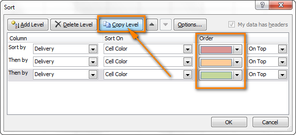
- In the Sort dialog window, specify the following settings from left to right.
- The column that you want to sort by (the Delivery column in our example)
- To sort by Cell Color
- Choose the color of cells that you want to be on top
- Choose On Top position

- Click the Copy Level button to add one more level with the same settings as the first one. Then, under Order, select the color second in priority. In the same way add as many levels as many different colors are in your table.
- Click OK and verify if your rows have got sorted by color correctly.
In our table, the "Past Due" orders are on top, then come "Due in" rows, and finally the "Delivered" orders, exactly as we wanted them.

Tip: If your cells are colored with many different colors, it is not necessary to create a formatting rule for each and every one of them. You can create rules only for those colors that really matter for you, e.g. "Past due" items in our example and leave all other rows in the current order.


If sorting cells by only one color is what you are looking for, then there's even a quicker way. Simply click on the AutoFilter arrow next to the column heading you want to sort by, choose Sort by color from the drop down menu, and then select the color of cells that you want to be on top or at the bottom. BTW, you can also access the "Custom Sort" dialog from here, as you can see in the right hand part of the screenshot below.

Sort cells by font color in Excel
In fact, sorting by font colour in Excel is absolutely the same as sorting by background color. You use the Custom Sort feature again (Home > Sort & Filter > Custom Sort…), but this time choose Font Color under "Sort on", as shown in the screenshot below.

If you want to sort by just one font color, then Excel's AutoFilter option will work for you too:

Apart from arranging your cells by background colour and font color, there may a few more scenarios when sorting by color comes in very handy.
Sort by cell icons
For example, we can apply conditional formatting icons based on the number in the Qty. column, as shown in the screenshot below.
![]()
As you see, big orders with quantity more than 6 are labeled with red icons, medium size orders have yellow icons and small orders have green icons. If you want the most important orders to be on top of the list, use the Custom Sort feature in the same way as described earlier and choose to sort by Cell Icon.
![]()
It is enough to specify the order of two icons out of 3, and all the rows with green icons will get moved to the bottom of the table anyway.
![]()
How to filter cells by color in Excel
If you want to filter the rows in your worksheet by colors in a particular column, you can use the Filter by Color option available in Excel 365 - Excel 2016.

The limitation of this feature is that it allows filtering by one color at a time. If you want to filter your data by two or more colours, perform the following steps:
- Create an additional column at the end of the table or next to the column that you want to filter by, let's name it "Filter by color".
- Enter the formula
=GetCellColor(F2)in cell 2 of the newly added "Filter by color" column, where F is the column congaing your colored cells that you want to filter by. - Copy the formula across the entire "Filter by color" column.

- Apply Excel's AutoFilter in the usual way and then select the needed colors in the drop-down list.


As a result, you will get the following table that displays only the rows with the two colors that you selected in the "Filter by color" column.

And this seems to be all for today, thank you for reading!
6 comments
"GETCELLCOLOR"
I have not any formula like that?
where can I find or add this formula?
Hello, Kaveh,
Please have a look at this article How to count and sum cells by color
WHen i enter the Getcellcolor formula it does not work. am i missing something?
Hello, John,
Please have a look at this article How to count and sum cells by color
Is there a possibility that we can sort two different colors in a single cell. e.g. First Name and Last Name are copied in a single cell, however, in different colors. Is there a way of sorting them? I hope, I made myself clear!
Hi Ankur,
The easiest way is to convert your data to an Excel table (select it and press Ctrl+T or click the Insert tab > Table). Then, simply click the Filter drop-down arrow in the Name column's header, choose Sort by Color and select the color you want to sort by. If you want to add sorting by a second color, then click Sort by Color > Custom Sort... > Copy Level and choose the second color.