Comparing columns in Excel is something that we all do once in a while. Microsoft Excel offers a number of options to compare and match data, but most of them focus on searching in one column. In this tutorial, we will explore several techniques to compare two columns in Excel and find matches and differences between them.
How to compare 2 columns in Excel row-by-row
When you do data analysis in Excel, one of the most frequent tasks is comparing data in each individual row. This task can be done by using the IF function, as demonstrated in the following examples.
Example 1. Compare two columns for matches or differences in the same row
To compare two columns in Excel row-by-row, write a usual IF formula that compares the first two cells. Enter the formula in some other column in the same row, and then copy it down to other cells by dragging the fill handle (a small square in the bottom-right corner of the selected cell). As you do this, the cursor changes to the plus sign:
To find cells within the same row having the same content, A2 and B2 in this example, the formula is as follows: To find cells in the same row with different values, simply replace the equals sign with the non-equality sign (<>): And of course, nothing prevents you from finding both matches and differences with a single formula: Or The result may look similar to this:
As you see, the formula handles numbers, dates, times and text strings equally well. Tip. You can also compare two columns row-by-row using Excel Advanced Filter. Here is an example showing how to filter matches and differences between 2 columns.
Formula for matches
=IF(A2=B2,"Match","")
Formula for differences
=IF(A2<>B2,"No match","")
Matches and differences
=IF(A2=B2,"Match","No match")=IF(A2<>B2,"No match","Match")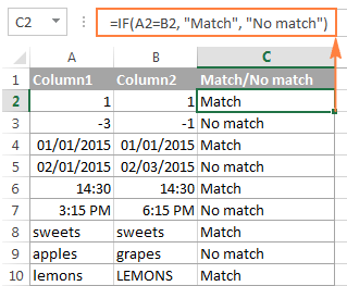
Example 2. Compare two lists for case-sensitive matches in the same row
As you have probably noticed, the formulas from the previous example ignore case when comparing text values, as in row 10 in the screenshot above. If you want to find case-sensitive matches between 2 columns in each row, then use the EXACT function:
=IF(EXACT(A2, B2), "Match", "")
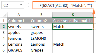
To find case-sensitive differences in the same row, enter the corresponding text ("Unique" in this example) in the 3rd argument of the IF function, e.g.:
=IF(EXACT(A2, B2), "Match", "Unique")
Compare multiple columns for matches in the same row
In your Excel worksheets, multiple columns can be compared based on the following criteria:
- Find rows with the same values in all columns (Example 1)
- Find rows with the same values in any 2 columns (Example 2)
Example 1. Find matches in all cells within the same row
If your table has three or more columns and you want to find rows that have the same values in all cells, an IF formula with an AND statement will work a treat:
=IF(AND(A2=B2, A2=C2), "Full match", "")
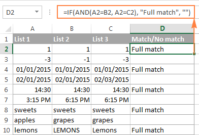
If your table has a lot of columns, a more elegant solution would be using the COUNTIF function:
=IF(COUNTIF($A2:$E2, $A2)=5, "Full match", "")
Where 5 is the number of columns you are comparing.
Example 2. Find matches in any two cells in the same row
If you are looking for a way to compare columns for any two or more cells with the same values within the same row, use an IF formula with an OR statement:
=IF(OR(A2=B2, B2=C2, A2=C2), "Match", "")
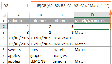
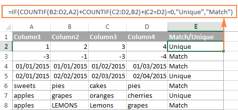
In case there are many columns to compare, your OR statement may grow too big in size. In this case, a better solution would be adding up several COUNTIF functions. The first COUNTIF counts how many columns have the same value as in the 1st column, the second COUNTIF counts how many of the remaining columns are equal to the 2nd column, and so on. If the count is 0, the formula returns "Unique", "Match" otherwise. For example:
=IF(COUNTIF(B2:D2,A2)+COUNTIF(C2:D2,B2)+(C2=D2)=0,"Unique","Match")
How to compare two columns in Excel for matches and differences
Suppose you have 2 lists of data in Excel, and you want to find all values (numbers, dates or text strings) which are in column A but not in column B.
For this, you can embed the COUNTIF($B:$B, $A2)=0 function in IF's logical test and check if it returns zero (no match is found) or any other number (at least 1 match is found).
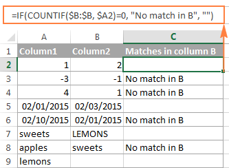
For instance, the following IF/COUNTIF formula searches across the entire column B for the value in cell A2. If no match is found, the formula returns "No match in B", an empty string otherwise:
=IF(COUNTIF($B:$B, $A2)=0, "No match in B", "")
Tip. If your table has a fixed number of rows, you can specify a certain range (e.g. $B2:$B10) rather than the entire column ($B:$B) for the formula to work faster on large data sets.
The same result can be achieved by using an IF formula with the embedded ISERROR and MATCH functions:
=IF(ISERROR(MATCH($A2,$B$2:$B$10,0)),"No match in B","")
Or, by using the following array formula (remember to press Ctrl + Shift + Enter to enter it correctly):
=IF(SUM(--($B$2:$B$10=$A2))=0, " No match in B", "")
If you want a single formula to identify both matches (duplicates) and differences (unique values), put some text for matches in the empty double quotes ("") in any of the above formulas. For example:
=IF(COUNTIF($B:$B, $A2)=0, "No match in B", "Match in B")
How to compare two lists in Excel and pull matches
Sometimes you may need not only match two columns in two different tables, but also pull matching entries from the lookup table. Microsoft Excel provides a special function for this - the VLOOKUP function. As an alternative, you can use a more powerful and versatile INDEX MATCH formula. The users of Excel 2021 and Excel 365, can accomplish the task with the XLOOKUP function.
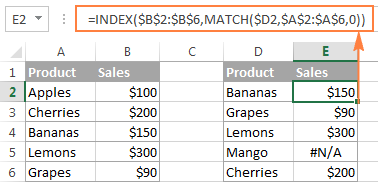
For example, the following formulas compare the product names in columns D against the names in column A and pull a corresponding sales figure from column B if a match is found, otherwise the #N/A error is returned.
=VLOOKUP(D2, $A$2:$B$6, 2, FALSE)
=INDEX($B$2:$B$6, MATCH($D2, $A$2:$A$6, 0))
=XLOOKUP(D2, $A$2:$A$6, $B$2:$B$6)
For more information, please see How to compare two columns using VLOOKUP.
If you don't feel very comfortable with formulas, you can have the job done using a fast and intuitive solution - Merge Tables Wizard.
Compare two lists and highlight matches and differences
When you compare columns in Excel, you may want to "visualize" the items that are present in one column but missing in the other. You can shade such cells in any color of your choosing by using the Excel Conditional Formatting feature and the following examples demonstrate the detailed steps.
Example 1. Highlight matches and differences in each row
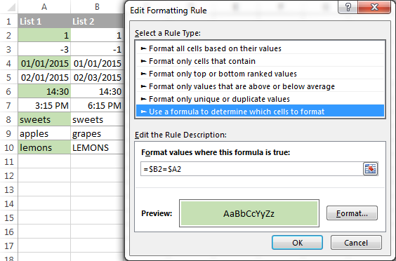
To compare two columns and Excel and highlight cells in column A that have identical entries in column B in the same row, do the following:
- Select the cells you want to highlight (you can select cells within one column or in several columns if you want to color entire rows).
- Click Conditional formatting > New Rule… > Use a formula to determine which cells to format.
- Create a rule with a simple formula like
=$B2=$A2(assuming that row 2 is the first row with data, not including the column header). Please double check that you use a relative row reference (without the $ sign) like in the formula above.
To highlight differences between column A and B, create a rule with this formula:
=$B2<>$A2
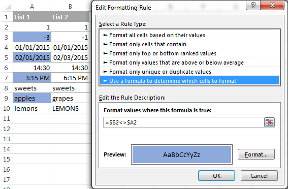
If you are new to Excel conditional formatting, please see How to create a formula-based conditional formatting rule for step-by-step instructions.
Example 2. Highlight unique entries in each list
Whenever you are comparing two lists in Excel, there are 3 item types that you can highlight:
- Items that are only in the 1st list (unique)
- Items that are only in the 2nd list (unique)
- Items that are in both lists (duplicates) - demonstrated in the next example.
This example demonstrates how to color the items that are only in one list.
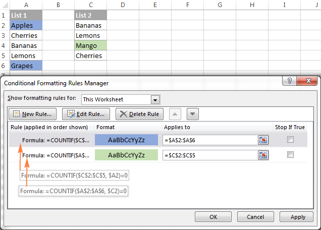
Supposing your List 1 is in column A (A2:A6) and List 2 in column C (C2:C5). You create the conditional formatting rules with the following formulas:
Highlight unique values in List 1 (column A):
=COUNTIF($C$2:$C$5, $A2)=0
Highlight unique values in List 2 (column C):
=COUNTIF($A$2:$A$6, $C2)=0
And get the following result:
Example 3. Highlight matches (duplicates) between 2 columns
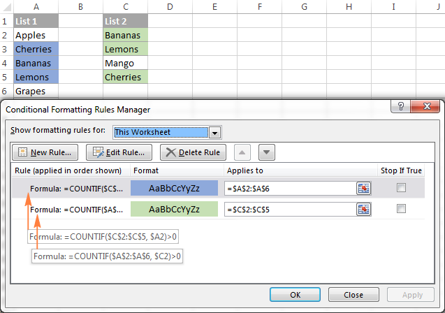
If you closely followed the previous example, you won't have difficulties adjusting the COUNTIF formulas so that they find the matches rather than differences. All you have to do is to set the count greater than zero:
Highlight matches in List 1 (column A):
=COUNTIF($C$2:$C$5, $A2)>0
Highlight matches in List 2 (column C):
=COUNTIF($A$2:$A$6, $C2)>0
Highlight row differences and matches in multiple columns
When comparing values in several columns row-by-row, the quickest way to highlight matches is creating a conditional formatting rule, and the fastest way to shade differences is embracing the Go To Special feature, as demonstrated in the following examples.
Example 1. Compare multiple columns and highlight row matches
To highlight rows that have identical values in all columns, create a conditional formatting rule based on one of the following formulas:
=AND($A2=$B2, $A2=$C2)
or
=COUNTIF($A2:$C2, $A2)=3
Where A2, B2 and C2 are the top-most cells and 3 is the number of columns to compare.
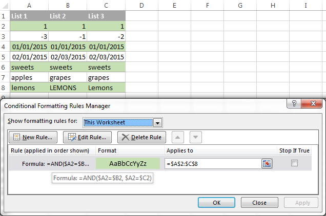
Of course, neither AND nor COUNTIF formula is limited to comparing only 3 columns, you can use similar formulas to highlight rows with the same values in 4, 5, 6 or more columns.
Example 2. Compare multiple columns and highlight row differences
To quickly highlight cells with different values in each individual row, you can use Excel's Go To Special feature.
- Select the range of cells you want to compare. In this example, I've selected cells A2 to C8.

By default, the top-most cell of the selected range is the active cell, and the cells from the other selected columns in the same row will be compared to that cell. As you can see in the screenshot above, the active cell is white while all other cells of the selected range are highlighted. In this example, the active cell is A2, so the comparison column is column A.
To change the comparison column, use either the Tab key to navigate through selected cells from left to right, or the Enter key to move from top to bottom.
Tip. To select non-adjacent columns, select the first column, press and hold Ctrl, and then select the other columns. The active cell will be in the last column (or in the last block of adjacent columns). To change the comparison column, use the Tab or Enter key as described above.
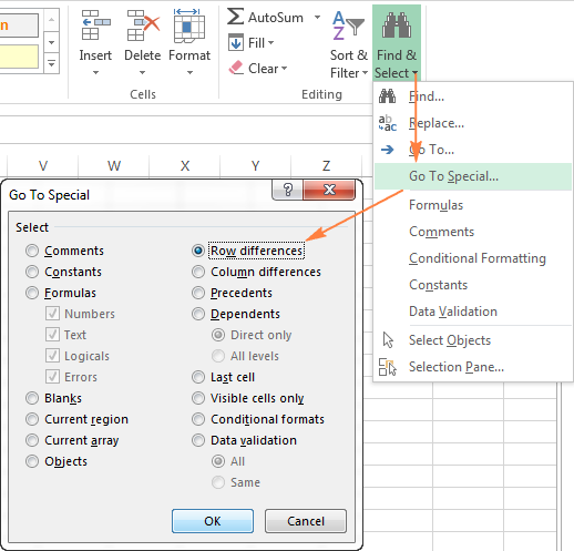
- On the Home tab, go to Editing group, and click Find & Select > Go To Special… Then select Row differences and click the OK button.
- The cells whose values are different from the comparison cell in each row are colored. If you want to shade the highlighted cells in some color, simply click the Fill Color icon on the ribbon and select the color of your choosing.

How to compare two cells in Excel
In fact, comparing 2 cells is a particular case of comparing two columns in Excel row-by-row except that you don't have to copy the formulas down to other cells in the column.
For example, to compare cells A1 and C1, you can use the following formulas.
For matches:
=IF(A1=C1, "Match", "")
For differences:
=IF(A1<>C1, "Difference", "")
To learn a few other ways to compare cells in Excel, please see:
Formula-free way to compare two columns / lists in Excel
Now that you know Excel's offerings for comparing and matching columns, let me show you our own solution for this task. This tool is named Compare Two Tables and it is included in our Ultimate Suite.
The add-in can compare two tables or lists by any number of columns and both identify matches/differences (as we did with formulas) and highlight them (as we did with conditional formatting).
For the purpose of this article, we'll be comparing the following 2 lists to find common values that are present in both.

To compare two lists, here are the steps you need to follow:
- Start with clicking the Compare Tables button on the Ablebits Data tab.

- Select the first column/list and click Next. In terms of the add-in, this is your Table 1.

- Select the second column/list and click Next. In terms of the add-in, it is your Table 2, and it can reside in the same or different worksheet or even in another workbook.

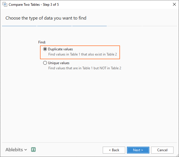
- Choose what kind of data to look for:
- Duplicate values (matches) - the items that exist in both lists.
- Unique values (differences) - the items that are present in list 1, but not in list 2.
Since our aim is to find matches, we select the first option and click Next.
- This is the key step where you select the columns for comparison. In our case, the choice is obvious as we are only comparing 2 columns: 2000 Winners against 2021 Winners. In bigger tables, you can select several column pairs to compare by.

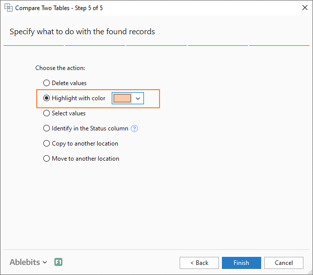
- In the final step, you choose how to deal with the found items and click Finish.
A few different options are available here. For our purposes, these two are most useful:
- Highlight with color - shades matches or differences in the selected color (like Excel conditional formatting does).
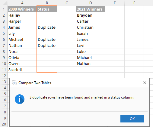
- Identify in the Status column - inserts the Status column with the "Duplicate" or "Unique" labels (like IF formulas do).
For this example, I've decided to highlight duplicates in the following color:
And in a moment, got the following result:

With the Status column, the result would look as follows:
Tip. If the lists you are comparing are in different worksheets or workbooks, it might be helpful to view Excel sheets side by side.
This is how you compare columns in Excel for matches (duplicates) and differences (unique values). If you are interested to try this tool, you are welcome to download an evaluation version using the below link.
I thank you for reading and encourage you to check out other helpful tutorials that we have :)
Available downloads
Compare Excel Lists - examples (.xlsx file)
Ultimate Suite - trial version (.exe file)
 by
by
546 comments
Hi I have beeen stuck in a problem I have data with mulipt column with simlier values but different lenght =INDEX($B$2:$B$6,MATCH($D2,$A$2:$A$6,0))
but problem is i have four columns withe common values in one two or three oe all four like your banan expmale so i want to extract the rspective values for common values in multiple columns how it will work tell me please or some other method
Its very good site, which is useful and saved my one week manual effort.
Regards,
Satish
I've been searching for a solution to this, but have so far haven't found an answer.
In a soccer league consisting of several matches there are a number of two differing outcomes to a specific criteria.
Here's a summary:
League and Result
ASIA: East Asian Championship Won
ASIA: East Asian Championship Lost
ASIA: East Asian Championship Women Lost
ASIA: East Asian Championship Women Won
AUSTRALIA: Brisbane Premier League Won
AUSTRALIA: Brisbane Premier League Lost
AUSTRALIA: Brisbane Premier League Won
AUSTRALIA: Brisbane Premier League Lost
AUSTRALIA: Brisbane Premier League Lost
AUSTRALIA: Brisbane Premier League Won
AUSTRALIA: Capital Territory Won
AUSTRALIA: Capital Territory Won
AUSTRALIA: Capital Territory Won
AUSTRALIA: Capital Territory Won
AUSTRALIA: Northern NSW Lost
AUSTRALIA: Northern NSW Won
AUSTRALIA: Northern NSW Lost
AUSTRALIA: Northern NSW Won
AUSTRALIA: Northern NSW Lost
AUSTRALIA: Northern NSW Won
AUSTRALIA: Northern NSW Lost
AUSTRALIA: Northern NSW Lost
What I want to do is create a report that lists each league and counts the number of Wins and Losses in each:
League Criteria
ASIA: East Asian Championship Won 1
ASIA: East Asian Championship Lost 1
ASIA: East Asian Championship Women Lost 1
ASIA: East Asian Championship Women Won 1
AUSTRALIA: Brisbane Premier League Won 3
AUSTRALIA: Brisbane Premier League Lost 3
AUSTRALIA: Capital Territory Won 4
AUSTRALIA: Northern NSW Lost 5
AUSTRALIA: Northern NSW Won 3
I've looked at Pivots, and that goes some of the way there. But I can't figure out how to count the number of wins and losses in each of the leagues.
Many thanks :)
row to row cheque the same the
numbar
hi....
I need a help to compare two sheets but it should compare the entire row only if there first column matches.
for example:
Sheet1
Row ID Order ID
32298 CA-2012-124891
26341 IN-2013-77878
25330 IN-2013-71249
13524 ES-2013-1579342
Sheet2
Row ID Order ID
32298 CA-2012-124891
26341 IN-2013-77878
25330 IN-2013-71249
here suppose row number 2,4,6 are blank or u can say contains other data. But need to compare row only when rowID matches...
32298==32298 but they are in different row numbers
Sorry, that earlier post was accident :)
Hi!
How can I make Excel sheet which compares Game result to my quess? And then I get points depends how good was my quess.
Here is small Example
Result My quess Points
0-1 0-2 4 winner right and one value right
1-1 1-1 10 Both values right = 10 points
1-1 2-1 0,5 One value right
1-2 0-3 3 Winner right, both values wrong
0-0 1-2 0 Both values wrong
Thanks very informative content
Hi can someone help me how i can compare two sheets columns and that compared cells has to be seen in other sheet. i consider it will very great i mean it may more visible
Hi, I need to show in a cell the number of rows that have value in any of the cells in it and give me the column titles.
example CFGA
3
because: there were three rows in the celection that had value only in columns CF and GA out of celected 4 columns.
Will greatly appreciate it.
Hi.. I would like to compare 2 different spread sheet data in excel. each spread sheet contains 15 columns and 1000 records. I would like to write a formula to know whether the spread sheet one data is matching with all the columns of spread sheet two or is there any change in each column. please let me know.
I would like to compare two different spreadsheets. The first spreadsheet has several names that are the same but with different criteria. Ex:
First column will have:
John Smith
John Smith
John Smith
John Smith
Peter Tom
Peter Tom
Peter Tom
Charlie Jones
Charlie Jones
Second column next to John Smith will have
Apples
Oranges
Pears
Bananas
On another worksheet I have John Smith then next to it Pears. What I want to do is to see if John Smith that has Pears is on the first worksheet.
Can anyone assist me?
how to get the sum for the folowing values in excel with out draging the mouse
ColumnA ColumnB ColumnC
1234 05:00
1234 03:30
1234 05:00
1234 03:30
1234 05:00
1234 03:30 =Totalhrs?
5678 05:00
5678 03:30
5678 05:00
5678 03:30
5678 05:00
5678 03:30 =Totalhrs ?
I want total hrs of 1234 and 5678 in columnC with some formulas urgent please
how to get the sum for the folowing values in excel with out draging the mouse
ColumnA ColumnB
1234 05:00
1234 03:30
1234 05:00
1234 03:30
1234
how to get the sum for the folowing values in excel with out draging the mouse
ColumnA ColumnB
1234
1234
1234
1234
1234
I'm trying to find how to write a formula for this scenario (pseudocode as follows): If Status="A" and dueDate contains a value, OR if Status = "C" (No dueDate info needed in this part), then it's True. Is there a way to have a formula order similar to If(OR((Status="C"),AND(Status="A",dueDate""),True, False))), or am I completely off track? Thank you in advance!
Hai
i have a big doubt to find the duplicate values and match the duplicate data's actual values
Hi ,
I wanted to find similar occurrences of string between two columns, If Column 1 text=Marks , then i need to find how many 'marks' in column 1 have 'pass' or 'fail' in column 2.
Thanks a TON!!!!!!
Thank you very much, these notes are really good and helpful for analysis.
Best,
Sameer
I need to sort column A where there is a duplicate number in red text. All numbers that don't have a duplicate red text number need to be removed.
Hello,
I am struggling with how to compare values, and if there is a match, insert a new column. For example, sheet 1 has:
Column A has server names, and will contain duplicates (column B contains application name, multiple app's can run on the same server)
Another spreadsheet (sheet 2) has unique server names by Datacenter (1 Excel sheet for each datacenter). I planned on copy/paste it into column D on sheet 1. If there is a match between column A and D, add a value (the value would be the same each time, as I am pasting only datacenter 1, then datacenter2, etc.) for the Datacenter into column C.
Hope that made sense, and thank you in advance!
I think I found a useable way to get this done, but not ideal. I'll compare the values, if it matches, write MATCH in column C. Then just replace the word MATCH with the Datacenter I am running it for. After a few runs, I'll be done, since I will paste one DC at a time. :-)
Hi,
can you please tell me how to take the difference of dates in cases like:
STARTTIME
24-MAR-16 09.25.20.859619000 AM
ENDTIME
24-MAR-16 09.25.23.028557000 AM
Hi!
I would like to check if the ask how to check two columns (one reference, one data) to another two columns even if they are not same in order. For example:
1) WORK 1 2) WORK 2
REFERENCE DATA REFERENCE DATA
001 RED 005 YELLOW
002 BLUE 001 RED
005 YELLOW 002 PINK
** REFERENCE 001 AND 005'S DATA ARE MATCH WITH WORK 2 DETAILS.
BUT FOR REFRENCE 002, DATAS ARE NOT MATCH WITH WORK 1 AND WORK 2
Even if they are not in the same order, by matching the reference and the data, I need to have a formula to know what details are not match for Work 1 to Work 2.
Please help me with this.
Thank you!
I wann compare this two colum in One Colum
Hi I want to compare just first 10 digits of the two cells.What formula can I use.
Did you find an answer for this Deeba? I need it too
Hi.. I have a data to sort.
As the numbers are not in sequence in each coloumn,
How can i make them in sequence to each other side by side.
Eg:
Column A Column B
211 212
212 214
213 215
214
215
What Im looking for is to sort column B data side by side with column A. I have 6000 numbers to sort right now.Thank you.
What it should be Eg:
Column A Column B
211
212 212
213
214 214
215 215
Sorry, I somehow posted before I was done writing..
I have two sets of data to compare: Column A to Column D, and Column B to Column E. How can I write one formula to look for matches or differences? For example:
Column A Column B Column C Column D Result
12345AA AEP 12345AA AEP True
12345AB AEP 12345SS HMA False
I hope this makes sense.
Thanks!
Liz
I have two sets of data to compare: Column A to Column D, and Column B to Column E. How can I write one formula to look for matches or differences? For example:
Column A Column B Column C Column D Result
12345AA AEP 12345AA AEP True
12345AB AEP
i have 2 columns a and b if the value of a and b column is "yes" the result should be displayed in c column as "resolved" but if either a or b has value no it should display as Followup,
i was able to apply the formula in c column but when the value of a column or a and b column both becomes no it displayes as false not the Followup what part i m missing
=IF(a:a="YES",IF(b:b="YES","Resolved","FOLLOWUP"))
Hi,
I have 6 digit alphanumeric data in Column A and B. Both are not in order and in different series. Few numbers in column A and B are same. how to find out common numbers in both column with a color highlight.
Thank you,
State Code
New Jersey NJ
New York NYC
Texas TX
If state is found in any where in the sheet.. the result should come in another column with state code.
State State
New Jersey
New Jersey
New Jersey
New York
Texas
New York
New Jersey
Texas
Texas
New Jersey
New Jersey
New Jersey
I want to keep index data with two columns (A, B) and find word in A in C column.. if A matches in C, add B in D column. Please help me with this.
Example:
Column A
New Jersey
Texas
New YORK
Column B:
NJ
TX
NYC
Column C:
New Jersey
New Jersey
New York
New Jersey
Texas
Texas
New York
New Jersey
Result should be in Column D:
NJ
NJ
NYC
NJ
TX
TX
NYC
NJ
Hi Dear
I have a problem to compare figure in the same row. How can i find out the row if the difference between them is more than double.
Great, Thanks a lot.
I need Example 3. Highlight matches (duplicates) between 2 columns for bank Reconciling because this problem
Column A Column B
2 match 2 Match
2 match
this case only one 2 match
Hi Irina Kindly give me your email so that I attach my illustrated problem.
Thanks in advance.
Hi Hermann,
You can send the description of your task with a sample spreadsheet to support@ablebits.com. Please include the name of the blog post and the number of your comment.
Please help me! I have 2 column a and b. "A" column have frutis information. "B" column have rates. The problem is a and b both have duplicate values. A have multiple time "orange". "B" have different rates sometime same rate. I have to find out does the orange has same rate all the time or different rate. If same rate than it has to display match if different rate. Than mismatch
Hello Gokul,
You can use our Duplicate Remover add-in:
https://www.ablebits.com/excel-suite/find-remove-duplicates.php
- Select your table and click on the Dedupe Table icon;
- Select columns A and B to compare rows of values;
- Choose the option to "Add the Status column"
The add-in will mark those rows that have the same fruit names with the same rates.
I need a mark to find duplicates in an excel sheet.
The problem with the records are, they are not exactly the same.
There is always one or more field(s) that differs from each other.
I want to have an automatic way of recognizing this cases.
Hello,
It sounds like our Fuzzy Duplicate Finder add-in will help you:
https://www.ablebits.com/excel-find-similar/index.php
It lets you specify the number of different characters and make the found values identical if necessary.
Hi all,
I would appreciate your help with the following:
I would like to compare two columns, let us say Column A and Column B, looking for duplicates. If a value in Column A has a match value in Column B, I would like to format the cells of the same duplicate value with the color (the colors are random and different for each match). This is if A12 = B30, the color will be red. And if A20 = B1, the color is green and so on.
Regards,
Ali
Hello Ali,
I'm sorry, but there is no simple way to do this. You can have a custom tool developed for you, but as soon as there are over ten values that have duplicates, you can only use the color shades that may be difficult to differentiate.
It may be better to create a conditional formatting rule to check duplicates of a particular value in column A and in column B, then change the rule to see the duplicates of the next value, and so on.
Hi, I need help with a formula. In my example, I am comparing dates between 2 columns (production dates), and I highlight only rows where the dates do not match. I wish to add to the existing formula, so that the comparison (and highlight) is not made if a third column is >1 (which would mean the order has already been produced). My intent is to focus on as-yet unproduced orders, and eliminate the highlight on orders already in stock.
Thank you!
Hi Joseph,
You can create a conditional formatting rule, choose to "Use a formula to determine which cells to format" and enter the following formula:
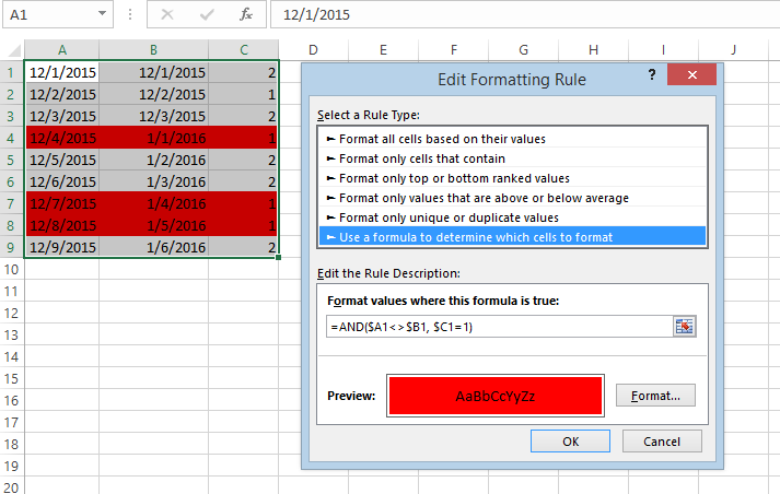
=AND($A1<>$B1, $C1=1)
Here columns A and B contain dates, and column C is the one to check for value "1":
Hi there, the article is very helpful, however I struggle with comparison where some empty cells are included.
Your "Compare multiple columns for matches in the same row" Example 1 is what I was searching for, but it doesn't work if there are empty cells in between.
Say A1= MARK, B1= MARK and C1 is empty, the function gives an error. How can I ignore those empty cells and still the answer to be "match".
Thanks!
Hello Yulia,
If blanks occur only in one of three values in the same row, please use the following formula:
=IF(AND(IF(AND(NOT(ISBLANK(A1)),NOT(ISBLANK(B1))), A1=B1, TRUE), IF(AND(NOT(ISBLANK(A1)),NOT(ISBLANK(C1))), A1=C1, TRUE), IF(AND(NOT(ISBLANK(C1)),NOT(ISBLANK(B1))), C1=B1, TRUE)), "Full match", "")
If you may have blanks in two of three values in the same row, please use this formula instead:
=IF(COUNTBLANK(A1:C1) > 1, "",IF(AND(IF(AND(NOT(ISBLANK(A1)),NOT(ISBLANK(B1))), A1=B1, TRUE), IF(AND(NOT(ISBLANK(A1)),NOT(ISBLANK(C1))), A1=C1, TRUE), IF(AND(NOT(ISBLANK(C1)),NOT(ISBLANK(B1))), C1=B1, TRUE)), "Full match", ""))
Hi Irina,
actually I have found another option: =IF(AND(OR(A1=B1;B1="");OR(A1=C1;C1=""));"ok";"error")
A little bit primitive, but for the purpose works good
Thanks
Yulia
how to check column 1 caste oc; column 2 male or female
how to count caste oc how many female and how many male ?
Hello Ram,
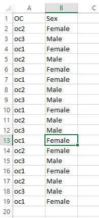
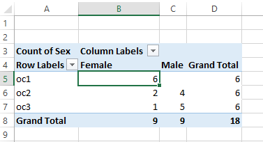
It sounds like you need to add a Pivot Table. We assume your data look the following way:
- Select your data, go to Insert tab in Excel and click on Pivot Table
- Drag column 1 to Rows
- Drag column 2 to Columns and to Values
You will get a count for each oc the following way:
Very useful. Very through. Fantastic
Thanks, the info was very helpful...
Helpul excel functions
Thanks.. helpful
I am wondering if possible to take column A make a match to the bestest (does not have to be 100% exact) match in column B and to say be able to copy that information back to where I want it to be. Doing some url links from data feed and testing idea's like this and hoping to come up with a better answer than doing it by hand. I got 519 rows in column A (menu name for links for website, etc) and 7546 rows in column B from data feed with the end to the links I want to make. Column A is say Women's Active Clothing Or Womens Active and Column B (has in the 7546 rows) a match like clothing & accessories > women > active (this is exact of how they look). I want to match them up then make a url out of it later like mysite.com/products/category/clothing & accessories > women > active to assign to menus like Women's Active Clothing. If any one has an idea please let me know. Am test trialing the software but yet not figured out or if possible to do some thing this hard
Hello, Rod,
For us to be able to assist you better, please send us a small sample table with your data in Excel and include the expected result. Thank you.
Need some help please. I have 3 separate cells, each ca contain variable data
e.g. Cells A1 and A2 can contain one of the following P, p, pi, pe,F, f, -, untested, Cell A3 can contain P,p,F,f,-,untested - what I want as a result in A4 is - If A1 and A2 and A3 all contain P or p(i or e also)then ALL OK, IF A1 or A2 or both contain an F or f but A3 = P or p then A4 should read T OK but prob. If Ai and A2 have P,p,pi,pe but A3 is F then A4 should read T OK up to x-point. If A1,A2 and A3 all contain an F or f then A4 should read T F
Hope you can help - Many Thanks
I've a problem in counting the number of appearing of the data in 2 adjcent cells in a same row.
Say the row is filled with alphabet randomly, I want to find the times that "B" appears immediately adjacent to "A".
Thank you.
Paul
Hello Paul,
Please try the formula below for your task.
=COUNTIF(A1:F1, "*AB*") + COUNTIF(A1:F1, "*BA*")
Hope this helps.
This was extremely helpful and thorough. Thank you!
it very useful