This tutorial explains the basics and beyond of the Excel time format.
Microsoft Excel has a handful of time features and knowing them in depth can save you a lot of time. To leverage powerful time functions, it helps to know how Excel stores times. In this article, you will find everything you need to know about formatting time in Excel:
Excel time format
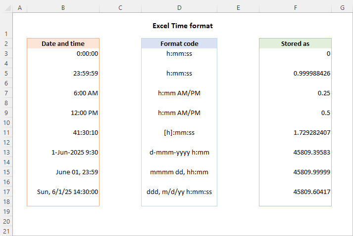
If you have been following our Excel Date Format tutorial, you know that Microsoft Excel stores dates as sequential numbers beginning with January 1, 1900, which is stored as number 1. As time is a portion of a day, times are stored as decimal fractions.
In Excel's internal system:
- 00:00:00 is stored as 0.0
- 23:59:59 is stored as 0.99999
- 06:00 AM is 0.25
- 12:00 PM is 0.5
When both date and time are entered in a cell, the value is stored as a decimal number comprised of an integer representing the date and a decimal portion representing the time. For example, 1 June 2025 9:30 AM is stored as 45809.39583.
How to get a decimal number representing time in Excel
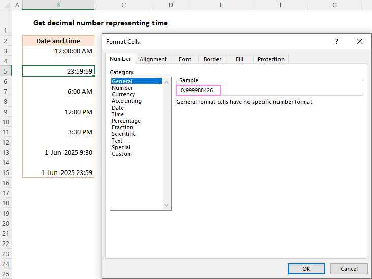
To get a decimal number representing a certain time, carry out these steps:
- Select a cell containing the time.
- Press Ctrl + 1 to open the Format Cells dialog box.
- On the Number tab, select General under Category, and you will see the decimal in the Sample box.
Now, you can write down that number and click Cancel to close the window. Or, you can click the OK button and have the time replaced with a corresponding decimal number in the cell.
To keep both the original time and its decimal representation, enter a simple formula like =B3 (where B3 is the time value) in any empty cell, and set the General number format for that cell.
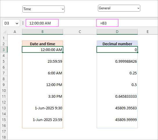
This is the fastest way to convert time to decimal in Excel. You can also use different formulas to convert time to hours, minutes or seconds.
How to format time in Excel
Microsoft Excel is smart enough to recognize a time value as you type it in a cell. For example, if you type 20:30, or 8:30 PM, or even 8:30 p, Excel will interpret this as a time and display either 20:30 or 8:30 PM, depending on your default time format.
To change an existing time formatting or apply some specific one, use the Format Cells dialog as described below.
- Select the cell(s) that you want to format.
- Press Ctrl + 1 to open the Format Cells dialog.
- On the Number tab, select Time from the Category list, and then choose the desired format from the Type list.
- Click OK to apply the selected format and close the dialog box.

Custom time format in Excel
Though Microsoft Excel provides a number of predefined time formats, you may want to create your own one that fits best for a particular sheet. This can also be done using the Format Cells dialog box:
- Select the target cells.
- Press Ctrl + 1 to open the Format Cells dialog.
- Under Category, select Custom and type the desired format code in the Type box.
- Review the Sample value to check if it's formatted as expected.
- Click OK to save the changes.
For example, to format a date time value like 1-Jun-2025 9:30 AM, utilize this code: d-mmm-yyyy h:mm AM/PM.

The custom time format you've created will be in the Type list the next time you need it.
Tip. The easiest way to make a custom time format is to use one of the existing formats as a starting point. For this, click Time in the Category list, and select one of the predefined formats under Type. After that switch to Custom and make the changes to the format displayed in the Type box.
Excel time formatting codes
When creating a custom time format in your worksheets, you can use the following codes.
| Code | Description | Displays as |
|---|---|---|
| h | Hours without a leading zero | 0-23 |
| hh | Hours with a leading zero | 00-23 |
| m | Minutes without a leading zero | 0-59 |
| mm | Minutes with a leading zero | 00-59 |
| s | Seconds without a leading zero | 0-59 |
| ss | Seconds with a leading zero | 00-59 |
| AM/PM | Periods of the day (if omitted, 24-hour time format is used) |
AM or PM |
12 hour time format in Excel
To set the 12 hour format for times in Excel, include AM/PM in the format code that you enter in the Format Cells dialog.
| Format | Displays as |
|---|---|
| h:mm:ss AM/PM | 1:30:00 PM |
| h:mm AM/PM | 1:30 PM |
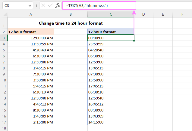
To change time to 12 hour format, you can also use the TEXT function with one of the codes listed above.
Assuming the original time value is in A3, the formula takes this form:
=TEXT(A3,"hh:mm:ss AM/PM")
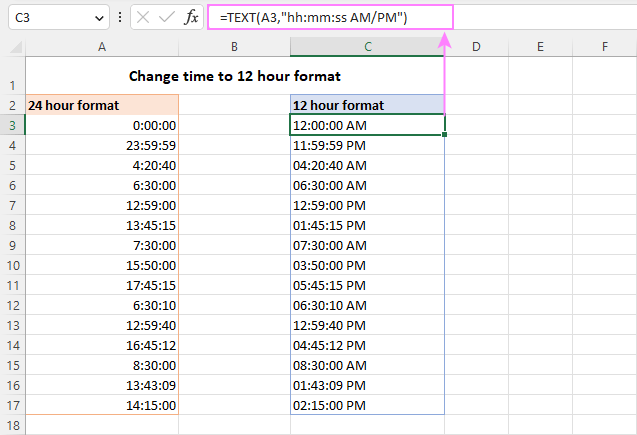
Note. The TIME function converts a time value into a text string. If you intend to calculate times at a later point, then set a custom 12-hour format using the Format Cells dialog.
24 hour time format in Excel
To apply the 24 hour time format, use any format code without AM/PM.
| Format | Displays as |
|---|---|
| h:mm:ss | 13:30:00 |
| h:mm | 13:30 |
Once you've decided on the format code, apply a corresponding custom format to the original cell or supply the format code to the TEXT function to return a formatted time in another cell. Remember that in the latter case, the output will be a text string.
With the source time in A3, the formula goes as follows:
=TEXT(A3,"hh:mm:ss")
Excel time format over 24 hours
When adding up times, the total may exceed 24 hours. To format times over 24 hours correctly, enclose the hour code in square brackets like [h].
Here are some examples of time formats over 24 hours:
| Format | Displays as | Explanation |
|---|---|---|
| [h]:mm | 41:30 | 41 hours and 30 minutes |
| [h]:mm:ss | 41:30:10 | 41 hours, 30 minutes and 10 seconds |
| [h] "hours", mm "minutes", ss "seconds" | 40 hours, 30 minutes, 10 seconds | |
| d h:mm:ss | 1 17:30:10 | 1 day, 17 hours, 30 minutes and 10 seconds |
| d "day" h:mm:ss | 1 day 17:30:10 | |
| d "day," h "hours," m "minutes and" s "seconds" | 1 day, 17 hours, 30 minutes and 10 seconds |
For more information, please see how to show, add, subtract over 24 hours, 60 minutes, 60 seconds.
Excel date time format
To create custom formatting for date and time, use various combinations of time and date format codes.
The following table provides some examples of how your Excel date time formats may look like:
| Format | Displays as |
|---|---|
| d-mmm-yy h:mm:ss AM/PM | 13-Jan-25 1:30:00 PM |
| mmmm dd, hh:mm AM/PM | January 13, 01:30 PM |
| dddd, m/d/yy h:mm:ss | Monday, 1/13/25 13:30:00 |
| ddd, mmmm dd, yyyy hh:mm | Mon, January 13, 2025 13:30 |
Excel time format without date
To format a date time value so that only time is visible in a cell, use only the time codes without the date codes. At that, you can use the international standard notation such as hh:mm:ss or your custom notation. Here are a few examples:
| Format | Displays as |
|---|---|
| h:mm:ss AM/PM | 1:30:00 PM |
| hh:mm:ss AM/PM | 01:30:00 PM |
| hh:mm:ss | 13:30:00 |
| hh-mm-ss | 13-30-00 |
| hh.mm.ss | 13.30.00 |
How to format negative time values
The custom time formats discussed above work for positive values only. If the result of your calculations is a negative number formatted as time (e.g. when you subtract a bigger time from a smaller one), the result will be displayed as #####. If you want to format negative time values differently, the following options are available to you:
- Display an empty cell for negative times. Type a semicolon at the end of the time format, for example [h]:mm;
- Display an error message. Type a semicolon at the end of the time format, and then type a message in quotation marks, e.g. [h]:mm;"Negative time"
Generally speaking, a semicolon acts as a delimiter to separate positive values' format from negative values' formatting. For full details, please see Custom Excel number format.
If you want to display negative times as negative values, e.g. -10:30, the easiest way is to switch to Excel's 1904 date system. For this, click File > Options > Advanced, scroll down to When calculating this workbook section and check the Use 1904 date system box.
For more information, please see How to calculate and display negative times in Excel.
Excel default time format
When setting up a time format in the Format Cells dialog, you may have noticed that one of the formats begins with an asterisk (*). This is the default time format in your Excel.

To quickly apply the default Excel time format to the selected cell or a range of cells, go to the Home tab > Number group, and choose Time from the Number Format drop-down list.
To change the default time format in Excel, this is what you need to do: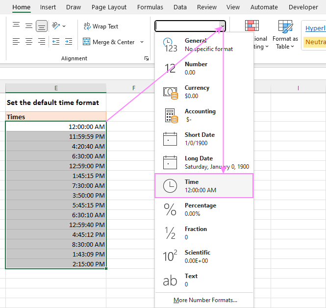
How to change the default time format

Now that you've got the hang of time formatting in Excel, it will be much easier for you to manipulate date and time values in your worksheets. I thank you for reading and hope to see you on our blog next week!
Practice workbook for download
Excel time formatting - examples (.xlsx file)
 by
by
165 comments
Hi,
If i want to display time format like 12:30 by typing 1230 only, which custom code should i use.
Hi! You can't automatically insert time separator after the second digit using the number format. This problem can be solved using VBA macro that can automatically do this and convert the value to a time. Read more: How to run macro in Excel and create a macro button.
If I want thousands of a second, in custom, use '.000'.
For example, my favorite detailed time format is: hh:mm:ss.000;@
Use '.000' for thousandths of a second,'.00' for hundredths, '.0' for tenths .
Microsoft mentions this in https://support.microsoft.com/en-us/office/format-numbers-as-dates-or-times-418bd3fe-0577-47c8-8caa-b4d30c528309
about 2/3rds of the way down is a table named 'Hours, minutes, and seconds'
The last item in the table is 'Fractions of a second'
sTART Time
Jan 1 2025 12:53PM
eND tIME
Jan 1 2025 3:21PM
HOW DO I FIND TOTAL TIME TAKE
Hi! You can find the examples and detailed instructions here: Calculate time in Excel: time difference, add, subtract and sum times
Hello Mr. Alexander
Can you give me formula regarding date/time difference between "August 8, 2024 13:00 and August 9, 2024 12:00" the column will show 23 hrs in difference..thank you
Hi! If I understand your task correctly, this article may be helpful: Calculate time in Excel: time difference, add, subtract and sum times.
If your date and time is written as text, then use these guidelines: How to convert text to date and number to date in Excel. Also use the TIMEVALUE function to convert text in time.
For the text “August 8, 2024 13:00” you can use a formula like this:
=DATE(MID(A1,FIND(",",A1)+2,4), VLOOKUP(LEFT(A1,3), {"JAN",1;"FEB",2;"MAR",3;"APR",4;"May",5;"JUN",6;"JUL",7;"AUG",8;"Sep",9;"OCT",10;"NOV",11;"DEC",12},2,0), SUBSTITUTE(MID(A1,FIND(" ",A1,1)+1,2),",","")) + TIMEVALUE(TRIM(RIGHT(SUBSTITUTE(A1," ",REPT(" ",LEN(A1))),LEN(A1))))
Going round in circles and finally admitting defeat. Have tried to summarise the data I am working with - this relates to hours worked for staff.
Col G Col H Col I Col M Col N Col O
Start Date Start Time Finish Time Start Time Finish Time Night hours
Format dd/mm/yyyy dd/mm/yyyy hh/mm AM/PM dd/mm/yyyy hh/mm AM/PM hh/mm/ss hh/mm/ss hh/mm/ss
24/07/2024 24/7/24 3:40AM 24/7/24 6:10AM 03:40:00 06:10:00
22/07/2024 22/7/24 11:45 PM 23/7/24 2:10AM 23:45:00 02:10:00
What I need to do in the night hours column (Col O) is account for any hours worked between midnight (23:59) and 6am (06:00). E.g. for the first Row should read 02:20 for 2hrs 20mins.
First thing i'm stuck on is i have used =TEXT(H2, "HH:MM:SS") in columns M and N to convert the date/time in H and I into time only. However - this isn't overwriting the original date in the underlying data, so every combination of IF statements that I try is giving false results.
I'm sure there is a very simple and straightforward answer, my brain is just fried. Thanks very much.
Hello Sharon!
There are several ways to extract the time from a cell that contains the date and time.
You can write the time in the cell as a text using the TEXT function and then you can convert this text into a time using the TIMEVALUE function. For example:
=TIMEVALUE(TEXT(A1,"HH:MM:SS"))
You can also use the mathematical function MOD:
=MOD(A1,1)
In the cell with the formula, set the time format you want.
Try to follow the recommendations from this article: Calculate time in Excel: time difference, add, subtract and sum times.
I hope it’ll be helpful. If something is still unclear, please feel free to ask.
Is it possible to display time units smaller than seconds in Excel, or do you have to roundup to the nearest second?
EG 2023-03-21 14:05:25.6960000
Hello Molly!
If you enter value using a formula bar, Excel cannot show milliseconds using time format. You can show milliseconds in a separate column.
If you get the time value using a formula, such as NOW function, you can use this time format:
dd.mm.yyyy h:mm.000
i have this raw data for day:hour:minit (without second), example 06:12:40 (6 days: 12 hours : 40 mins) how do i put this in excel format so that i can use it in a formula. thanks
Hi! You can use Text to Columns tool:
1. Select the data range containing your times.
2. Go to the "Data" tab and click "Text to Columns"
3. In the Text to Columns Wizard choose "Delimited" and click "Next."
4. Set delimiter between day, hour, and minute ":"
5. Choose "General" as the data format for all columns and click "Finish"
To extract time from your text string using formula, you can extract all characters starting from the fourth character using MID function and convert them to time as described in this guide: Convert text to time using TIMEVALUE function.
=TIMEVALUE(MID(A1,4,20))
=TIMEVALUE(MID(A1,SEARCH(":",A1)+1,20))
SEARCH function finds the position of the first ":" in the text string to separate the number of days.
You can extract the number of days using the LEFT function:
=VALUE(LEFT(A1,SEARCH(":",A1)-1))
VALUE function converts text to a number.
how to convert 1h 30m 4.1s to 01:30:04?
Hi! Determine the position of the decimal point with the SEARCH function and delete the extra digits of the seconds with the LEFT function.
Replace the hour and minute symbols "h " and "m " with ":" in the text string using the SUBSTITUTE function.
Convert the resulting text string to time using the TIMEVALUE function.
Based on this information, the formula could be as follows:
=TIMEVALUE(SUBSTITUTE(SUBSTITUTE(LEFT(A1,SEARCH(".",A1)-1),"h ",":"),"m ",":"))
hello, im trying to convert 991:00:00 = 10/02/1900 07:00:00 into a number 991. How can I do it?
Hello! If your value is written as time, use the TEXT function and these instructions: Show time over 24 hours, 60 minutes, 60 seconds in Excel.
=TEXT(A1,"[h]")
You will get a text string that you can convert to a number as described here: How to convert text to number in Excel.
For example:
=--TEXT(A1,"[h]")
I have a result generated from from google form test in excel as 31/40 and I want the results presented as 31. How can I go about it? My regards.
Hi! If your result is a text string, you can extract the desired characters using these instructions: Get text before a specific character. For example:
=LEFT(A1,SEARCH("/",A1)-1)
It is not possible to show only part of the text string in a cell using formatting.
Is there any way to use a format like:
YEARS:MONTHS:DAYS:MINUTES:SECONDS ?
In an amount of time way, not a date way.
Hi! If you want to find the difference in dates and times, try using the DATEDIF function:
=DATEDIF(0, A1-B1, "y") &" years, "&DATEDIF(0, A1-B1, "ym") &" months, " &DATEDIF(0, A1-B1, "md") &" days "&INT(MOD(A1-B1,1)*24)&" h "&MOD(MOD(A1-B1,1)*24,1)*60&" m "
or
=DATEDIF(0, A1-B1, "y") &" : "&DATEDIF(0, A1-B1, "ym") &" : " &DATEDIF(0, A1-B1, "md") &" : "&INT(MOD(A1-B1,1)*24)&" : "&MOD(MOD(A1-B1,1)*24,1)*60
A1 -end date & time. B1 - start date & time
You can find the examples and detailed instructions here: Excel DATEDIF to calculate date difference in days, weeks, months or years. You can also find useful information in this article: How to convert time to decimal number, hours, minutes or seconds in Excel.
I am looking to convert a number (stored in seconds) to h:mm:ss format
example:
A1 = 3510 A2 = =CONVERT(Q397,"sec","mn") formated as general with a result of 58.5
I am trying to have the 58.5 show as 58.30 or 58:30 ( 58 mins and 30 seconds).
Hi! You can convert seconds to minutes using these formulas. In the cell with the formula, set the custom time format to "mm:ss".
=CONVERT(Q397,"sec","mn")/1440
=Q397/60/1440
=Q397/60/60/24
Please take a look at this guide: How to convert numbers to time format in Excel.
Is there a way to show a elapsed time, such as 145:24:37 as 145:25, without changing the actual value or using formulas?
Hi! You must use number rounding formulas to round time. You can't do this using the time format.
I'm using the [h]:mm format.
Shift start time today 4,:00 AM to shift end time next day 4:00 AM, based on the shift start and end time only I need to calculate time utilizes, pl help me to get results through formula
Cell : A : 04,:00:00 20-Dec-2023
Cell: B: 04:21:00 21-Dec-223
Hi! If you have the date and time written in your cells, just find their difference as described in this guide: Calculate time in Excel: time difference, add, subtract and sum times.
If this does not work for you, please describe the problem and your data in more detail.
We cannot change format of this text string 13/04/2023 07:40:15 to date & time in excell
Hi! I don't know what local date and time format you use. But I think the recommendations in this article will help you solve the problem: How to convert text to date and number to date in Excel. If this does not help, explain the problem in more detail.
I have questions on excel regarding a What formula I should use?
Ending 02:00:00 AM - 03:00 (hours) = 11:00:00 PM (results)
Result Cell is formatted in Time
You can find the answer to your question in this article: Calculate time in Excel: time difference, add, subtract and sum times.
Dear sir, is it possible to mention time in From-To format in MS excel, for ex. 5:00am to 6:00am or 5:00 to 6:00.
If yes then how, Please help me with this.
Hi!
To perform time calculations, each time value must be written to a separate cell. You can concatenate these values into a text string, as described in this tutorial: Excel CONCATENATE function to combine strings, cells, columns.
Good morning,
Trying to textjoin 2 cells containing time in one, (i.e 5:00 and 13:00), but the format i get is a number (0,208333-0,54166) and i want format in time again. Trying =TEXT(C2;HH:MM) but the result is a message (Excel ran out of resources while trying to calculate one or more formulas)
Hi!
Use the TEXT function for each of the time values you are concatenating.
=TEXT(C1;"HH:MM")&" - "&TEXT(C2;"HH:MM")
I want to calculate TAT. It is mentioned in the excel as 20-11-2022 15:52:17, its a start time and end time 20-11-2022 15:52:20. I have to calculate this where I should know how much days required along with time. How to do this.
I have used formula =TEXT(AB2-AA2,"h:mm:ss") to arrived on the time. Which later i have converted in hours with formula =HOUR(AC2)+MINUTE(AC2)/60
But i want it together as how to calculate if its beyond any day. please help
Hi!
If I understand your task correctly, the following tutorial should help: How to calculate time in Excel - time difference, adding / subtracting times.
Hi,
Please what I want is adding a difference of 4 hours to the initial time. Let's say my current time is 8:00 amin column A, I want to create a formula to automatically calculate time in the next 4 hours (i.e. 12:00 pm) in the next column B.
How do I do this on excel?
Hello!
The following tutorial should help: Adding or subtracting hours, minutes and seconds to a time.
Please convert this "1 day 21 hours 3 minutes " in to this " 40:03:00" or "1 day 56 minutes into "24:56:00" or "1 minute " into "00:01:00"