The tutorial explains how to use multiple IF in Excel and provides a couple of nested If formula examples for most common tasks.
If someone asks you what Excel function you use most often, what would your answer be? In most cases, it's the Excel IF function. A regular If formula that tests a single condition is very straightforward and easy to write. But what if your data requires more elaborate logical tests with multiple conditions? In this case, you can include several IF functions in one formula, and these multiple If statements are called Excel Nested IF. The biggest advantage of the nested If statement is that it allows you to check more than one condition and return different values depending on the results of those checks, all in a single formula.
Microsoft Excel has limits to the levels of nested IFs. In Excel 2003 and lower, up to 7 levels were allowed. In Excel 2007 and higher, you can nest up to 64 IF functions in one formula.
Further on in this tutorial, you will find a couple of Excel nested If examples along with a detailed explanation of their syntax and logic.
Example 1. Classic nested IF formula
Here's a typical example of Excel If with multiple conditions. Supposing you have a list of students in column A and their exam scores in column B, and you want to classify the scores with the following conditions:
- Excellent: Over 249
- Good: between 249 and 200, inclusive
- Satisfactory: between 199 and 150, inclusive
- Poor: Under 150
And now, let's write a nested IF function based on the above criteria. It's considered a good practice to begin with the most important condition and keep your functions as simple as possible. Our Excel nested IF formula goes as follows:
=IF(B2>249, "Excellent", IF(B2>=200, "Good", IF(B2>150, "Satisfactory", "Poor")))
And works exactly as it should:
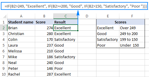
Understanding Excel nested IF logic
I've heard some people say that Excel multiple If is driving them crazy :) Try looking at it at a different angle:

What the formula actually tells Excel to do is to evaluate the logical_test of the first IF function and, if the condition is met, return the value supplied in the value_if_true argument. If the condition of the 1st If function is not met, then test the 2nd If statement, and so on.
IF(check if B2>=200, if true - return "Good", or else
IF(check if B2>150, if true - return "Satisfactory", if false -
return "Poor")))
If you need a nested IF formula with wildcard characters (partial match), check out this example: If cell contains, then return different values.
Example 2. Multiple If with arithmetic calculations
Here's another typical task: the unit price varies depending on the specified quantity, and your goal is to write a formula that calculates the total price for any amount of items input in a specific cell. In other words, your formula needs to check multiple conditions and perform different calculations depending on what amount range the specified quantity falls in:
| Unit Quantity | Price per unit |
| 1 to 10 | $20 |
| 11 to 19 | $18 |
| 20 to 49 | $16 |
| 50 to 100 | $13 |
| Over 101 | $12 |
This task can also be accomplished by using multiple IF functions. The logic is the same as in the above example, the only difference is that you multiply the specified quantity by the value returned by nested IFs (i.e. the corresponding price per unit).
Assuming the user enters the quantity in cell B8, the formula is as follows:
=B8*IF(B8>=101, 12, IF(B8>=50, 13, IF(B8>=20, 16, IF( B8>=11, 18, IF(B8>=1, 20, "")))))
And the result will look something similar to this:
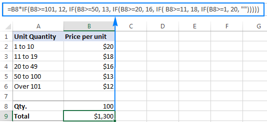
As you understand, this example demonstrates only the general approach, and you can easily customize this nested If function depending on your particular task.
For example, instead of "hard-coding" the prices in the formula, you can reference the cells containing those values (cells B2 to B6). This will enable your users to edit the source data without having to update the formula:
=B8*IF(B8>=101,B6, IF(B8>=50, B5, IF(B8>=20, B4, IF( B8>=11, B3, IF(B8>=1, B2, "")))))
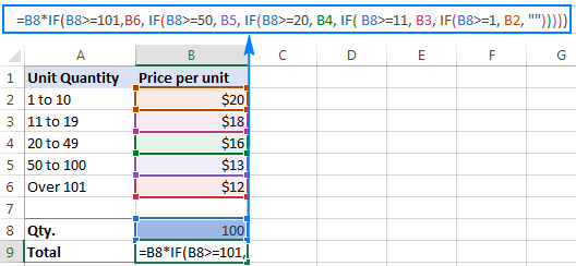
Or, you may want to include an additional IF function(s) that fixes an upper, lower or both bounds of the amount range. When the quantity is outside the range, the formula will display an "out of the range" message. For example:
=IF(OR(B8>200,B8<1), "Qty. out of range", B8*IF(B8>=101,12, IF(B8>=50, 13, IF(B8>=20, 16, IF( B8>=11, 18, IF(B8>=1, 20, ""))))))
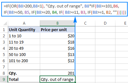
The nested IF formulas described above work in all versions of Excel. In Excel 365 and Excel 2021, you can also use the IFS function for the same purpose.
Advanced Excel users that are familiar with array formulas, can use this formula that basically does the same thing as the nested IF function discussed above. Though the array formula is far more difficult to comprehend, let along to write, it has one indisputable advantage - you specify the range of cells containing your conditions rather than referencing each condition individually. This makes the formula more flexible, and if your users happen to change any of the existing conditions or add a new one, you will only have to update a single range reference in the formula.
Excel nested IF - tips and tricks
As you have just seen, there is no rocket science in using multiple IF in Excel. The following tips will help you improve your nested IF formulas and prevent common mistakes.
Nested IF limits
In Excel 2007 - Excel 365, you can nest up to 64 IF functions. In older versions of Excel 2003 and lower, up to 7 nested IF functions can be used. However, the fact that you can nest a lot of IFs in one formula doesn't mean you should. Please keep in mind that each additional level makes your formula more difficult to understand and troubleshoot. If your formula has too many nested levels, you may want to optimize it by using one of these alternatives.
The order of nested IF functions matters
The Excel nested IF function evaluates the logical tests in the order they appear in the formula, and as soon as one of the conditions evaluates to TRUE, the subsequent conditions are not tested. In other words, the formula stops after the first TRUE result.
Let's see how it works in practice. With B2 equal to 274, the nested IF formula below evaluates the first logical test (B2>249), and returns "Excellent" because this logical test is TRUE:
=IF(B2>249, "Excellent", IF(B2>=200, "Good", IF(B2>150, "Satisfactory", "Poor")))
Now, let's reverse the order of IF functions:
=IF(B2>150, "Satisfactory", IF(B2>200, "Good", IF(B2>249, "Excellent", "Poor")))
The formula tests the first condition, and because 274 is greater than 150, the result of this logical test is also TRUE. Consequently, the formula returns "Satisfactory" without testing other conditions.
You see, changing the order of IF functions changes the result:

Evaluate the formula logic
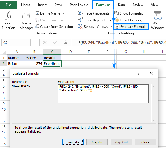
To watch the logical flow of your nested IF formula step-by-step, use the Evaluate Formula feature located on the Formula tab, in the Formula Auditing group. The underlined expression is the part currently under evaluation, and clicking the Evaluate button will show you all the steps in the evaluation process.
For example, the evaluation of the first logical test of the nested IF formula shown in the screenshot below will go as follows: B2>249; 274>249; TRUE; Excellent.
Balance the parenthesis of nested IF functions
One of the main challenges with nested IFs in Excel is matching parenthesis pairs. If the parentheses do not match, your formula won't work. Luckily, Microsoft Excel provides a couple of features that can help you to balance the parentheses when editing a formula:
- If you have more than one set of parentheses, the parenthesis pairs are shaded in different colors so that the opening parenthesis matches the closing one.
- When you close a parenthesis, Excel briefly highlights the matching pair. The same bolding, or "flickering", effect is produced when you move through the formula by using the arrow keys.

For more information, please see Match parenthesis pairs in Excel formulas.
Treat text and numbers differently
When building logical tests of your nested IF formulas, remember that text and numbers should be treated differently - always enclose text values in double quotes, but never put quotes around numbers:
Right: =IF(B2>249, "Excellent",…)
Wrong: =IF(B2>"249", "Excellent",…)
The logical test of the second formula will return FALSE even if the value in B2 is greater than 249. Why? Because 249 is a number and "249" is a numeric string, which are two different things.
Add spaces or line breaks to make nested IFs easier to read
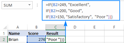
When building a formula with multiple nested IF levels, you can make the formula's logic clearer by separating different IF functions with spaces or line breaks. Excel doesn't care about extra spacing in a formula, so you may not worry about mangling it.
To move a certain part of the formula to the next line, just click where you want to insert a line break, and press Alt + Enter. Then, expand the formula bar as much as needed and you will see that your nested IF formula has become much easier to understand.
Alternatives to nested IF in Excel
To get around the limit of seven nested IF functions in Excel 2003 and older versions and to make your formulas more compact and fast, consider using the following alternatives to nested Excel IF functions.
- To test multiple conditions and return different values based on the results of those tests, you can use the CHOOSE function instead of nested IFs.
- Build a reference table and a use VLOOKUP with approximate match as shown in this example: VLOOKUP instead of nested IF in Excel.
- Use IF with logical functions OR / AND, as demonstrated in the these examples.
- Use an array formula like shown in this example.
- Combine multiple IF statements by using the CONCATENATE function or the concatenate operator (&). A formula example can be found here.
- For experienced Excel users, the best alternative to using multiple nested IF functions might be creating a custom worksheet function using VBA.
This is how you use an If formula in Excel with multiple conditions. I thank you for reading and hope to see you on our blog next week.
Practice workbook for download
Nested If Excel statements (.xlsx file)
 by
by
635 comments
I want to know how to calculate incentive for employees based on the below slab
Sale Range Incentive
0 - 2 lakh 0% ( Minimum level )
2 - 2.5 Lakh 10%
2.5 - 3 Lakh 15%
3 - 3.5 Lakh 20%
If the total sale is 2.75 lakh we have to give the employee an incentive for the amount of 75,000(2.75 lakh - 2.00 lakh ) . Out of the 75000, 50000 will be under 10% and balance 25000 will fall under 15% category. Can you help me to find a formula to calculate the incentive amount.
Hello!
Such questions have already been asked on the blog. I recommend reading this answer and this comment.
I hope my advice will help you solve your task.
If D2 is less than or equal to zero then G2 is equal to C2 plus .05, the rest is the same
If D2 is less than or equal to zero then G2 is equal to C2, or if D2 is greater than zero then G2 is equal to C2
Sorry I made a mistake. if D2 then G2 is equal to C2
I need excel to keep/change values in G2. If D20 then I want it to record the same value that is in C2
Hi!
I’m sorry but your task is not entirely clear to me. What does the condition "If D20" mean? Please describe your problem in more detail.
I am trying to use 2 if statements in 1 cell.
if H2 = Y THEN I2 WILL = E AND IF H2 = N THEN I2 WILL = F
How can I write this in a formula. I have tried everything and cant get it to work.
Thank you
carissa
Hello!
If I understand your task correctly, the following formula should work for you:
=IF(H2="Y","E",IF(H2="N","F",""))
Hope this is what you need.
I have a data set on multiple row;
A1 40
A2 80
A3 60
A4 30
Is there any way I can use if condition to see A1:A4 >=40 in one take, rather that each if condition check for individual row?
Thank you.
Hello!
Explain what result you would like to get?
IF(Data)>F$1,F$1,(Data))
Can anyone explain, what comes from it and how?
if debit days 0-31 or security=2 month ,"5%",if security=1 month ,"4","3".and other condition is if debit days 31-62 or security=2 month,"4.5",if security=1 month,'3','1.5'. how can we use if formula
Hi
I've looked across this page trying to find a solution to my problem i have learnt a lot, tried many examples and with adaptions but keep getting errors.
I'm querying a cell entry, there would be a possible 10 entries but need to show something different in another cell.
problem - (if_C1=###,then###,or###,then###)
So if the data in C1=FCP-1 THEN IN CELL J1 SHOW !F1, BUT if C1=FCP-2 then in J1 show !F2 and so on.
any help would be appreciated.
Kind regards,
G
Hello!
I’m sorry but your task is not entirely clear to me. For me to be able to help you better, please describe your task in more detail. Please specify what you were trying to find, what formula you used and what problem or error occurred. Give an example of the source data and the expected result.
It’ll help me understand it better and find a solution for you. Thank you.
I am trying to enter a code that says if text is in the P column on row 4 then the $ amount entered in Q column row 4 would be automatically entered into a merged cell column K/L lines 4-7. I can't figure it out. Can you help me with that?
Hello Sue!
If I got you right, the formula below will help you with your task:
=IF(P4<>"",Q4,"")
Write this formula in merged cell column K/L lines 4-7
Hi
I have a bus having seater size 40 and customer price is 100 below slab and want to calculate the Amount earn by A & B :-
Occupancy A share % B Share % Amount A earn Amount B earn
SLAB 1 20% 100% 0%
30% 100% 0%
40% 100% 0%
50% 100% 0%
60% 100% 0%
SLAB 2 60.1% 60% 40%
65% 60% 40%
70% 60% 40%
75% 60% 40%
80% 60% 40%
SLAB 3 80.1% 10% 90%
85% 10% 90%
90% 10% 90%
95% 10% 90%
100% 10% 90%
Hello!
I’m sorry but your task is not entirely clear to me. For me to be able to help you better, please describe your task in more detail. Explain your details. Please specify what you were trying to find, what formula you used and what problem or error occurred. It’ll help me understand it better and find a solution for you. Thank you.
I reviewed several formulas, entry level, and couldn't find one to do the following: compare three numbers, select the lowest of the three and once selected to input a text outcome.
Ex: 115000/Low 125000/Median 130000/High
They are in different boxes but on same row. G21, J21 & N21 with the text to be written on say P21. Could someone please direct me to a proper formula that I can use. Thank You!!
Hello Eve!
For me to be able to help you better, please specify which formula you mean and describe the problem in more detail. Are only numbers or numbers and text written in the cells? Do you want to display the minimum value in some other cell? Or want to select a cell with a minimum value? What does "text to be written on say P21" mean? Thank you.
dear,
please solve this,
if i take some figures total in need how many times coming actual coming
for ex:
120+128+126+59+596+1669+1556 = 4254
now i need how many times coming 600 in 4254 so need formula in excel
thanks and regards
Hello Rinash!
If I understand your task correctly, the following formula should work for you:
=INT(4254/600)
Read more in this article.
Hope this is what you need.
I am using the following: =IFERROR(VLOOKUP($F5,ndapo,$E5)+30,($F5-150)*VLOOKUP($F5,ndappo,$E5)+VLOOKUP($F5,ndapo,$E5))
It works with the exception that it doesn't add the per pound rate. Example:
column References: F=Bill Wgt; ndapo=net rates; e=Zone
Rated Zone Bill WGT rate with no per lb rates
108 225 $1,276.50
108 225 $1,281.20
My goal:
150lb Rate <150 rate Per lbs Excess Wgt <150 Total Per lbs Result should be
$1,246.50 8.31 75 $623.25 $1,869.75
Hello Gabriela!
I'm sorry, it is not very clear what result you want to get. Could you please describe your task in more detail? What is the ndapo named range (or ndappo?) Or send us a small sample workbook with the source data and expected result to support@ablebits.com? Please shorten your tables to 5-10 rows/columns and include the link to your blog comment.
We'll look into your task and try to help.
I'm hoping someone can help with this. I'm trying to calculate a timesheet (working Hours), but if someone has annual leave. I want to be able to calculate the annual leave, with leave loading, without typing a start and finish time. just 'AL' in the start time cell and it'll calculate the 8hrs with the workers pay rate. because there are different pay rates.
this is the formula i started but it only calculates the first day and no more 'AL' in that week. PLEASE HELP
=IF(ISERROR(A8),"",IF(B8="AL",AP8*1.175*8,IF(I8="AL",AP8*1.175*8,IF(P8="AL",AP8*1.175*8,IF(W8="AL",AP8*1.175*8,IF(AD8="AL",AP8*1.175*8,SUM(AK8*AP8)))))))
Hello Jack!
I'm sorry, it is not very clear what result you want to get. Could you please describe your task in more detail and send us a small sample workbook with the source data and expected result to support@ablebits.com? Please shorten your tables to 10-20 rows/columns and include the link to your blog comment.
We'll look into your task and try to help.
Hi,
Hope you can help me with this. I want to return a result for a cell called "Risk Class" based on a text value of "severity" and "probability". Depending on the combinations of "severity" and "probability" the following "Risk Class" results should be presented. Hope someone can come up with the relevant nested IF?
using the formula
If severity = L and Probability = L then Risk Class = 3
severity Probability = Risk Class
L L = 3
hi,
i am getting trouble in if statement
i have more then 300 product code with there values so if i multiple code by more than 64 steps it doesn't count any one suggest me what to do ?
example .
=IF(AM29=441,H29*46,IF(AM29=443,H29*13,IF(AM29=48119,H29*21,IF(AM29=48111,H29*427,IF(AM29=48112,H29*483,IF(AM29=48122,H29*581,IF(AM29=48211,H29*150,IF(AM29=48212,H29*193,IF(AM29=48213,H29*76,IF(AM29=48221,H29*167,IF(AM29=48222,H29*217,IF(AM29=48231,H29*177,IF(AM29=48232,H29*224,IF(AM29=41611,H29*1305,IF(AM29=4919,H29*3023,IF(AM29=49111,H29*3561,IF(AM29=4721,H29*7,IF(AM29=4722,H29*8,IF(AM29=4724,H29*6,IF(AM29=4712,H29*9,IF(AM29=4713,H29*6,IF(AM29=41022,H29*1644,IF(AM29=41023,H29*1737,IF(AM29=41025,H29*2256,IF(AM29=41026,H29*2333,IF(AM29=410210,H29*2960,IF(AM29=41637,H29*331,IF(AM29=41031,H29*511,IF(AM29=41034,H29*404,IF(AM29=41042,H29*314,IF(AM29=41043,H29*320,IF(AM29=41046,H29*101,IF(AM29=4151,H29*13,IF(AM29=4833,H29*114,IF(AM29=4834,H29*144,IF(AM29=4832,H29*186,IF(AM29=4911,H29*644,IF(AM29=4915,H29*4040,IF(AM29=4120,H29*32,IF(AM29=511,H29*192,IF(AM29=512,H29*229,IF(AM29=513,H29*232,IF(AM29=514,H29*250,IF(AM29=614,H29*334,IF(AM29=613,H29*244,IF(AM29=616,H29*182,IF(AM29=618,H29*165,IF(AM29=565,H29*19,IF(AM29=412213,H29*250,IF(AM29=412214,H29*269,IF(AM29=412212,H29*174,IF(AM29=41233,H29*570,IF(AM29=543,H29*102,IF(AM29=544,H29*132,IF(AM29=545,H29*66,IF(AM29=4116,H29*1877,IF(AM29=4117,H29*1963,IF(AM29=4925,H29*247,IF(AM29=525,H29*77,IF(AM29=531,H29*214,IF(AM29=532,H29*199,IF(AM29=533,H29*260,IF(AM29=445,H29*1928,IF(AM29=446,H29*2333,IF(AM29=447,H29*3203,"")))))))))))))))))))))))))))))))))))))))))))))))))))))))))))))))))
Hello Abid!
I'm sorry, it is not very clear what result you want to get. Could you please describe your task in more detail and send us a small sample workbook with the source data and expected result to support@ablebits.com? Please shorten your tables to 10-20 rows/columns and include the link to your blog comment.
We'll look into your task and try to help.
Thank you! This is exactly what I needed to sort out my IF formula!
Hi,
Please help me to solve this
Deposits Lots Category
150,000 1,750 Platinum
50,000 1,000 Gold
25,000 200 Silver
If both Column A & B satisfied the respective category should be displayed.
Thanks in advance
Help! I need a formula that helps with the following:
I have an average formula in a cell G4 (averaging B4:F4)
I need to have a functional formula that does:
If G4 is between 1.0-1.5, then 1
If G4 is between 1.6-2.5, then 2
If G4 is between 2.6-3.5, then 3
If G4 is greater than 3.6, then 4
I am getting "False" forthis formula.
Advice on how to correct it please ?
=IF(AND(AF2="Incomplete",BE2=""),"Not Done",IF(AND(AF2="Negative",BE2=""),"Negative",IF(AND(AF2="Positive",BE2=BE2:BE5),"Done")))
So I use to work for a company that I helped them out with replacing parts on their machines when it got within a certain date range. I did this using excel and its the only one that I did. I currently working on something similar where lets say there is an end date of 1-6-2020 and I need a formula that gives me a red flag when the actual date gets within 30 days of that June Date. I can't remember how the formula goes. could anyone give me a little bit of advice?
Assuming the end date is entered in A1:
=IF(TODAY()+30>=A1,"Deadline coming up","Still enough time")
=IF(H2>=$F$1;IF(H1="NED";"NE";IF(H1>=$F$1;"DA";));"NE")
i need to add another IF- if it is "SUB" then "NE"
(H1="NED";"NE";IF(H1>=$F$1;"DA";));"NE")-> this but with SUB, and it needs to fit in the formula on the top
pleeeease
Hey I need some help, is it possible to fetch the below data with formula.
I have a length formula in column b which is returning various values from col A. 17,14,13
In case of 17 i have two arguments to check simultaneously,
1. check the 4th character if it is "-" (hyphen) then mid(5,10)
2.check the 14th character if it is "-" (hyphen) then mid(4,10)
in case of 14 i have 4 arguments to check simultaneously,
1. look for 4 character to be "-"(hyphen), then need right(10)
2. look for 4 character to be " "(space), then need right(10)
3. look for 11 character to be "-"(hyphen), then left(10)
4. look for 1 character to be "*"(star shift8), then right(10)
in case of len 13 2 arguments
1. look for 11 character to be "-"(hyphen), then left(10),
2. right(10)
Can all the above arguments can happen with 1 if function starting in column c
Please help
Amazing !!!!
Excellent !!!
Great !!!
Hello,
I am attempting to figure out a formula for accessing lieu and vacation time accumulated and taken.
If an employee has used up all lieu and I need time taken to start drawing from vacation what would be the formula?
E.g. Employee has 15 lieu hours and 30 vacation hours.
They take 16 hours off.
The time has to come off lieu first then pull from vacation.
Hi,
I have a query, the below works but I need it to cover two ranges B38@B57 and G38:G57 rather than just the individual cells in each case, but when I input that I get #VALUE!
Can anyone advise?
=IF(B38="","Available",IF(G38="","Off Sick",IF(B38="",G38="","Available2")))
Many thanks
HI,
I have a question, I want to do a calculation for Logistics (Port Storage charges) these amounts changes every few days. The Number of days in port I have however how to calculate the following in af formula?
From day 1 until day 11 = USD 0,00 per day
From day 12 until day 20 = USD. 2.00 per day
From day 21 until day 40 = USD 9.00 per day
From day 41 until day 70 = USD 25.00 per day
Over 70 days = USD 42 per day
Hi,
I have the following formula that works fine:
=SUM(IF(G4="Rad",4,IF(G4="Green",3,IF(G4="Blue",2,IF(G4="Yellow",1,Good))))/COUNTA(G4:J4))
where
Red = 4
Green =3
Blue = 2
and Yellow 1
are a selection from dropdown list to calculate a percentage based on the selection.
I want to apply this formula for entire row.
what I did is below:
=SUM(IF(G4="Rad",4,IF(G4="Green",3,IF(G4="Blue",2,IF(G4="Yellow",1))))
+(IF(H4="Rad",4,IF(H4="Green",3,IF(H4="Blue",2,IF(H4="Yellow",1))))
+(IF(I4="Rad",4,IF(I4="Green",3,IF(I4="Blue",2,IF(I4="Yellow",1))))
+(IF(J4="Rad",4,IF(J4="Green",3,IF(J4="Blue",2,IF(J4="Yellow",1))))/COUNTA(G4:J4))
It will be hard if have 30 or 50 cells,
so is there a way to do it by selecting the range instead and each cell manual
condition 1 = Sum Insured
condition 2 = Age Bracket
Result = Premium
How to input the formula?
Premium given in excel sheet in different row according to age bracket
Is it possible to abbreviate the formula when non-consecutive numbers are used? I have a sheet where I need to assign 12 department numbers to one of three groups, with a 4th group as a catch all for outliers. The department numbers are not sequential.
So for instance can I say IF(B2=(211,224,266,267),"Group A",IF(B2=(286,216),"Group B",IF(B2=(210,268,288,270,218,225),"Group C","Group D")))) it doesn't work. Do I need to write out a really long formula with all possibilites? What would that look like?
I cant do thes if statement
cash back
example 1 amount 5000 70
example 2 amount 6500 110
from to of amount max to give
1000– 3000 1% 30
4,000 - 6000 2% 80
6,000 - 10000 4% 240
10,000 - 15000 7% 700
15,000 - Open 12% 1800
My result returns #VALUE! how do I get around that?
=IF('ADPR -AWARDS KDG L J TRANSITION'!L10<19000,'ADPR -AWARDS KDG L J TRANSITION'!A10*'ADPR -AWARDS KDG L J TRANSITION'!F10,0),IF('Benef Ovr Grid'!E3,'ADPR -AWARDS KDG L J TRANSITION'!L10-19000,0)
need an if statement that uses if c2 starts with '00' rather than typing out long names
I am grading a test and some questions have multiple answers and the answers are two characters. How do I look up answer (NM) in cell A1 and (ND) in cell B1 to the answer key that had (NM) in cell M1 and (ND) in cell N1? In order to be correct, both answers (NM &ND) have to be provided and does not have to be in any order. An I do this with an If then statement?
I have a spreadsheet calculating months of service to clients. They can have a start date, a suspended date, a restart date and an exit date. The service may have never been suspended so the suspended date and the restart date could be empty. There could be a suspended date and never restart so the exit would be the same as the suspended date. I am trying to calculate the total months of service to each client. How can I write an if/or statement to tell it to use start date then suspended date then restart date then exit date, but to ignore there is no suspended date, but to use start and suspend date if there is no restart date? This is what I have so far: =(DATEDIF(D2,E2,"D")+DATEDIF(F2,I2,"D"))/30
Hi, I would like to kindly request some assistance.
Is there any formula that can select a few cells below a VLookup result if a certain condition is met? Example VLOOKUP result is cell D10 but if the amount in cell E10 is >1, then the Vlookup should pull the result in cell D15. Appreciate any advice. Thank you so much
I need TO USE IF CONTIONS WITH 15 CONTIONS HOW I CAN GET WIHT TEXTS
I need TO USE IF CONTIONS WITH 15 CONTIONS HOW I CAN GET
Hello, Im looking to insert a nested IF function but only on blank cells of a column. Any idea?
I Know how to fill out blank spaces with a value, but not with a formula.
Thanks in advance!
Need help to select items from column A with respect to range of items available in D column using if function.
=if(A:A=range excluded plants,"YES","NO")
PLANT Excluded Plants
1 1052
2 1014
3 1033
4 1015
5 1018
6 1017
7
8
9
1014
Any help would be appreciated, i want to look at a cell and if it meets the criteria of GMBH or INC INC then it looks up the cell reference otherwise returns N/A but cant' get it to work.
=IF(D708="GMBH",IF(D708-"INC", VLOOKUP('2018 Margin Data'!A$1:A$65536,'Master Margin'!$A$4:$T$983,17,0),"N/A"))
I have an excel sheet in which "C1" column is "MODEL" & "D1" column is "LANDING".
Another side I have created a list of MODELS in "Q1" column & LANDING PRICE in "R1" column.
I want a formula...that if I type a model number in column "C2" landing will automatically will put in column "D2"
I have an excel sheet in which "C1" column is "MODEL" & "D1" column is "LANDING".
Another side I have created a list of MODELS in "Q1" column & LANDING PRICE in "R1" column.
I want a formula...that if I type a model number in column "C2" landing will automatically will put in column "D2"
And If I type any model number in the column "C2" landing price automatically will come to the column number "D2"
Hi, I have two conditional parameters..
The simple formula is: =IF(F19<=15; F18*F19*72; IF(F1930; F19*F18*72*0,91)))
Where:
F19 is number of days.
F18 is number of cats.
But I need another one when is more then 1 cat, so for each extra cat the value is $20, and not the same price of one. How do I work a formula with more then one condition parameter?
Hi,
Is there a way to write the formula below in Excel? The percentage ranges are column headings not individual cells.
=if(B6 is greater than 5% but less than 10%,E4,if(B6(greater than 10% then F2,if(B6 is less than 5%, B3,error)))
Hi
I'm hoping you can help me with a formula for this
if A1:A2="","" if A1="" & A2 = X,"O" if A1:A2 = X,"X"
I need to do a formula that will look at a range of columns on a specific row and if a value then give data from that column with value row 2, where the column with value is different row.
I have 2 sheets in excel, the first carrying the data and the second where the data will be placed. I am to compute the fuel consumption of the different types of equipment however there are types of equipment in the first sheet which has the same dates and have to be added together in a single cell in the 2nd sheet. Which formula should I use to compute it?
=IF(H39>99,"5000",IF(H39>89,"4500", IF(H39>79,"4000", IF(H39>69,"3500",IF(H39>59,"3000", IF(H39>49,"2500",IF(H39>39,"2000", IF(H39>29,"1500", IF(H39>19,"1000", IF(H39>9,"500","NOT ELEGIBLE"))))))))))
I have made a formula to conduct screening work from data and that is
=IF(J13=167.64;30;IF(J13=168.91;32.5;IF(J13=170.18;35;IF(J13=171.45;37.5;IF(J13=172.72;40;IF(J13=173.99;42.5;IF(J13=175.26;45;IF(J13=176.53;47.5;J13>=177.8;50)))))))))
but it shows that the formula is too large.
how can I reduce it.
Seeking help from any one.
I think the issue you are having is you are using ";" to separate you if statement. You should us "," instead. Let me know if this works for you.
James