 by
by The tutorial shows how to combine VLOOKUP and IF function together to v-lookup with if condition in Excel. You will also learn how to use IF ISNA VLOOKUP formulas to replace #N/A errors with your own text, zero or blank cell.
Whilst the VLOOKUP and IF functions are useful on their own, together they deliver even more valuable experiences. This tutorial implies that you remember the syntax of the two functions well, otherwise you may want to brush up on your knowledge by following the above links.
Vlookup with If statement: return True/False, Yes/No, etc.
One of the most common scenarios when you combine If and Vlookup together is to compare the value returned by Vlookup with a sample value and return Yes / No or True / False as the result.
In most cases, the following generic formula would work nicely:
Translated in plain English, the formula instructs Excel to return True if Vlookup is true (i.e. equal to the specified value). If Vlookup is false (not equal to the specified value), the formula returns False.
Below you will a find a few real-life uses of this IF Vlookup formula.
Example 1. Look up a specific value
Let's say, you have a list of items in column A and quantity in column B. You are creating a dashboard for your users and need a formula that would check the quantity for an item in E1 and inform the user whether the item is in stock or sold out.
You pull the quantity with a regular Vlookup with exact match formula like this:
=VLOOKUP(E1,$A$2:$B$10,2,FALSE)
Then, write an IF statement that compares Vlookup's result with zero, and returns "No" if it is equal to 0, "Yes" otherwise:
=IF(VLOOKUP(E1,$A$2:$B$10,2,FALSE)=0,"No","Yes")
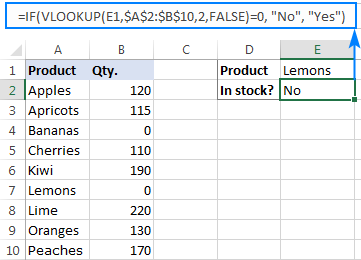
Instead of Yes/No, you can return TRUE/FALSE or In Stock/Sold out or any other two choices. For example:
=IF(VLOOKUP(E1,$A$2:$B$10,2)=0,"Sold out","In stock")
You can also compare the value returned by Vlookup with sample text. In this case, be sure to enclose a text string in quotation marks, like this:
=IF(VLOOKUP(E1,$A$2:$B$10,2)="sample text",TRUE,FALSE)
Example 2. Compare Vlookup result with another cell
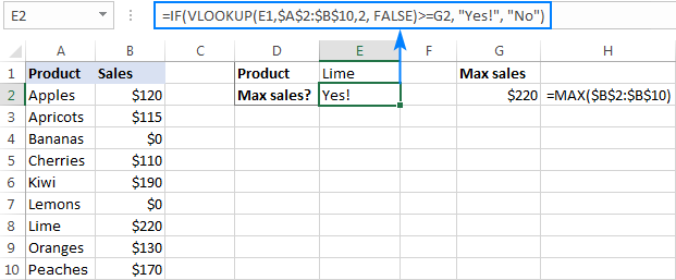
Another typical example of Vlookup with If condition in Excel is comparing the Vlookup output with a value in another cell. For example, we can check if it's greater than or equal to a number in cell G2:
=IF(VLOOKUP(E1,$A$2:$B$10,2)>=G2,"Yes!","No")
And here is our If formula with Vlookup in action:
In a similar fashion, you can use any other logical operator together with a cell reference in your Excel If Vlookup formula.
Example 3. Vlookup values in a shorter list
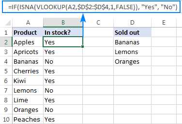
To compare each cell in the target column with another list and return True or Yes if a match is found, False or No otherwise, use this generic IF ISNA VLOOKUP formula:
If Vlookup results in the #N/A error, the formula returns "No", meaning the lookup value is not found in the lookup list. If the match is found, "Yes" is returned. For example:
=IF(ISNA(VLOOKUP(A2,$D$2:$D$4,1,FALSE)),"No","Yes")

If your business logic requires the opposite results, simply swap "Yes" and "No" to reverse the formula's logic:
=IF(ISNA(VLOOKUP(A2,$D$2:$D$4,1,FALSE)),"Yes","No")
Excel If Vlookup formula to perform different calculations
Besides displaying your own text messages, If function with Vlookup can perform different calculations based on the criteria you specify.
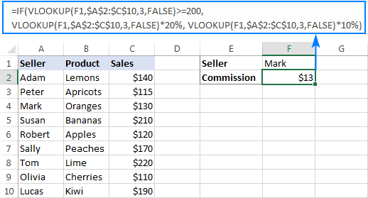
Taking our example further, let's calculate the commission of a specific seller (F1) depending on their effectiveness: 20% commission for those who made $200 and more, 10% for everyone else.
For this, you check if the value returned by Vlookup is greater than or equal to 200, and if it is, multiply it by 20%, otherwise by 10%:
=IF(VLOOKUP(F1,$A$2:$C$10,3,FALSE )>=200, VLOOKUP(F1,$A$2:$C$10,3,FALSE)*20%, VLOOKUP(F1,$A$2:$C$10,3,FALSE)*10%)
Where A2:A10 are seller names and C2:C10 are sales.
IF ISNA VLOOKUP to hide #N/A errors
If the VLOOKUP function cannot find a specified value, it throws an #N/A error. To catch that error and replace it with your own text, embed a Vlookup formula in the logical test of the IF function, like this:
Naturally, you can type any text you like instead of "Not found".
Supposing, you have a list of seller names in one column and sales amounts in another column. Your task is to pull a number corresponding to the name the user enters in F1. If the name is not found, display a message indicating so.
With the names in A2:A10 and amounts C2:C10, the task can be fulfilled with the following If Vlookup formula:
=IF(ISNA(VLOOKUP(F1,$A$2:$C$10,3,FALSE)), "Not found", VLOOKUP(F1,$A$2:$C$10,3,FALSE))
If the name is found, a corresponding sales amount is returned:

If the lookup value is not found, the Not found message appears instead of the #N/A error:

How this formula works
The formula's logic is very simple: you use the ISNA function to check Vlookup for #N/A errors. If an error occurs, ISNA returns TRUE, otherwise FALSE. The above values go to the logical test of the IF function, which does one of the following:
- If the logical test is TRUE (#N/A error), your message is displayed.
- If the logical test is FALSE (lookup value is found), Vlookup returns a match normally.
IFNA VLOOKUP in newer Excel versions
Beginning with Excel 2013, you can use the IFNA function instead of IF ISNA to catch and handle #N/A errors:
In our example, the formula would take the following shape:
=IFNA(VLOOKUP(F1,$A$2:$C$10,3, FALSE), "Not found")
Tip. If you'd like to trap all sorts of errors, not only #N/A, use VLOOKUP in combination with the IFERROR function. More details can be found here: IFERROR VLOOKUP in Excel.
Excel Vlookup: if not found return 0
When working with numerical values, you may want to return a zero when the lookup value is not found. To have it done, use the IF ISNA VLOOKUP formula discussed above with a little modification: instead of a text message, supply 0 in the value_if_true argument of the IF function:
In our sample table, the formula would go as follows:
=IF(ISNA(VLOOKUP(F2,$A$2:$C$10,3,FALSE)), 0, VLOOKUP(F2,$A$2:$C$10,3,FALSE))

In the recent versions of Excel 2016 and 2013, you can use the IFNA Vlookup combination again:
=IFNA(VLOOKUP(I2,$A$2:$C$10,3, FALSE), 0)
Excel Vlookup: if not found return blank cell
This is one more variation of the "Vlookup if then" statement: return nothing when the lookup value is not found. To do this, instruct your formula to return an empty string ("") instead of the #N/A error:
Below are a couple of complete formula examples:
For all Excel versions:
=IF(ISNA(VLOOKUP(F2,$A$2:$C$10,3,FALSE)), "", VLOOKUP(F2,$A$2:$C$10,3,FALSE))
For Excel 2016 and Excel 2013:
=IFNA(VLOOKUP(F2,$A$2:$C$10,3, FALSE), "")

If with Index Match - left vlookup with If condition
Experienced Excel users know that the VLOOKUP function is not the only way to do vertical lookup in Excel. The INDEX MATCH combination can also be used for this purpose and it's even more powerful and versatile. The good news is that Index Match can work together with IF in exactly the same way as Vlookup.
For example, you have order numbers in column A and seller names in column B. You are looking for a formula to pull the order number for a specific seller.
Vlookup cannot be used in this case because it cannot search from right to left. Index Match will work without a hitch as long as the lookup value is found in the lookup column. If not, a #N/A error will show up. To replace the standard error notation with your own text, nest Index Match inside IF ISNA:
=IF(ISNA(INDEX(A2:A10, MATCH(F1, $B$2:$B$10, 0))), "Not found", INDEX(A2:A10, MATCH(F1, $B$2:$B$10, 0)))
In Excel 2016 and 2016, you can use IFNA instead of IF ISNA to make the formula more compact:
=IFNA(INDEX(A2:A10, MATCH(F1, $B$2:$B$10, 0)), "Not found")

In a similar manner, you can use Index Match in other If formulas.
This is how you use Vlookup and IF statement together in Excel. To have a closer look at the formulas discussed in this tutorial, you are welcome to download our sample workbook below. I thank you for reading and hope to see you on our blog next week!
Practice workbook for download
Excel IF Vlookup - formula examples (.xlsx file)
Latest comments
How do I display data from a different column on the same row when VLOOKUP provides a match? For instance, I want to compare column D on sheet 1 to column H on sheet 2 and display the data from sheet 2 column C from the same row on sheet 1. I used the following: =IF(VLOOKUP(D2,'sheet2'!H:H,1,FALSE)=D2,'sheet2'!C7). The problem is that it is not displaying the data from sheet 2 column C for the corresponding row for sheet 2 column H. It s displaying column C in order. I need to perform this on several rows of data.
Hi! If I understand your task correctly, the following tutorial should help: Left lookup with INDEX MATCH. Hope this is what you need.
Hi, I would like to pull in the billed fee amount from a different data set if the unique matter number and the name of the client manager matches. Accordingly, there are two conditions: 1) matter number 2) Client manager.
Your support is greatly appreciated.
Thanks in advance.
Hello Sarah!
You can find the examples and detailed instructions here: Excel INDEX MATCH with multiple criteria - formula examples
I have a monthly time sheet for a single staff member in South Africa. Her hours are flexible and that makes the tax rate differ monthly.
Once I have her monthly figure from the hours worked I need to refer to a table provided by SARS (tax) and if her earnings are between X and Y then I choose that value.
How do I set up my excel to automatically access the table (I have retyped the rows/columns that would be relevant (base remuneration, top remuneration, tax rate). So for example:
If she earned R9287 in the month I would look at the table row where the salary falls between R9222 and R9322 and select the tax figure of R233.
I would like the system to do this for me. HELP.
Thanks.
Hello Janet!
To check that a number is within a certain interval, use approximate match. We have special tutorials on this. Please see: How to Vlookup for approximate match and Approximate match XLOOKUP.
The data you have provided is not enough to offer you a formula.
Good morning,
This might not be possible and I'm struggling to search for it properly to find an answer and I hope I'm not confusing this too much, but I basically want a formula which uses the data in one cell to return a specific result, and if it doesn't match I want it to then vlookup to a specific range on a data sheet (so if the data in one cell matches it overrides the need to do the vlookup function, but if it doesn't match then it reverts to the vlookup) :
If data in Cell H12 = a certain phrase then return a specific text result.
But if the phrase doesn't match, then I want it to run through an if/or vlookup (I already have this formula and it works fine (below), but I want it to use the above condition as the primary source to return a result.
So the if/or vlookup formula I am using successfully is: =IF(OR($J$9="N",(VLOOKUP($F$16,Dropdowns!$G$4:$K$117,5,0))),"",VLOOKUP($F$16,Dropdowns!$G$4:$K$117,5,0))
But was then trying to also incorporate =IF($H$12="Service","Manager")
So if "Service" is selected from a drop down box in one cell, it returns "Manager" in the cell I want, but if a different option is selected like "Sales" or "Marketing" etc then it reverts to using the vlookup formula above to determine who the budget holder/approver would be.
Apologies, that probably all sounds a mess.
Many thanks!
Hi! If my understanding is correct, the following formula should work for you:
=IF($H$12="Service","Manager", IF(OR($J$9="N",(VLOOKUP($F$16,Dropdowns!$G$4:$K$117,5,0))),"",VLOOKUP($F$16,Dropdowns!$G$4:$K$117,5,0)))
Maybe this article will be helpful: Nested IF in Excel – formula with multiple conditions.
I am trying to create a new reference column in a data set to say 'If cell from column B is found in the lookup table, then return text from cell B + cell E, otherwise return just the value/text from cell B' - It is working for some, but not others.
Can you help?
=IF(VLOOKUP(B11,$N$9:$N$12,1,TRUE)=B11,TEXTJOIN(" - ",,B11,E11),B11)
Hi! If the value B11 is not found, the VLOOKUP function will return an error. Use the IFERROR function to return only the B11 value in case of an error. Try this formula:
=IFERROR(TEXTJOIN(" - ",,VLOOKUP(B11,$N$9:$N$12,1,TRUE),E11),B11)
Hi,
I have a data set where in one column i have unique code, which needs to be mapped/looked-up in another tab but the data required is in multiple tables and i need to lookup that data based on the priority .
Example "qt3213e" is my unique key which can be available in more then 1 table but based on my priority is should 1st search in table 2 then table 1 and so on till it is found and return the value in front of it. How can this be done. Thanks.
Hi! You can use different VLOOKUP formulas depending on the cell value. You can use the nested IF formula or the IFS function for this purpose. For example:
=IFS(C1=1, VLOOKUP(......),C1=2, VLOOKUP( ........))
Hello
i have 12 seet of 12 month and i want to make one master seet all seet have pary name and its payble amount , for exampale , we have to do 2000 payment to abcd party in jan. And 3000 in feb. How can i make master seet to seet all month payment in row, i want formula that put jan paybale ammount in jan cell ,not in diffrent month cell .
So please help me with make this master seet
Thank you.
Hello! Unfortunately, this information is not enough to recommend a formula to you. I don't really understand how your data is organized. I hope this instruction will be helpful: INDEX MATCH MATCH in Excel for two-dimensional lookup.
Hi I am hoping to use excel to drive an advice action
Column 2 = drop down list
Column 3 = will return a text based action based on the response in Column 2
For example:
drop down = yes => Talk to Mel
drop down = no => leave blank
drop down = not sure => Talk to Sam
drop down = [any other choice] => Further information required
Hi!
Here is the article that may be helpful to you: How to make a dependent (cascading) drop-down list in Excel
Hi, I would like a formula for the below criteria
I have two sheets, the first fixed one contains the restaurant names with their fixed delivery charge in the column next to them, E.g Restaurant A (delivery charge 10), Restaurant B (delivery charge is 12), etc..
The second sheet will contain the deliveries done for the month. So if the name of the restaurant matches its equivelant name in the first sheet, then the delivery charge is 10. If the second row also has restaurant A then charge is 10 again, if third row contains restaurant B, then delivery charge is 12.
Thank you
Hi!
You can find the answer to your question in this article: How to VLOOKUP across multiple sheets in Excel.
I would need help on the following conditions please if possible.
If Column A meet the criteria and Column B meet another criteria, return Column C.
But if the Column C is blank, look for the next return value under Column C where Column A & B still both meets the criteria.
Hi!
If I understand your task correctly, the following tutorial should help: Excel INDEX MATCH with multiple criteria.
You have three criteria - for A, for B, and for C - the cell is not empty.
Hi, I need exactly what describe in the scenario of "Vlookup with If statement: return True/False, Yes/No, etc." With only one twist.
Imagine I have multiple rows of "Lemons" in column A with different values (10,6,etc) and I need the function to tell me true/false only if one of the "Lemon" rows hits the value of "0" value in column B ignoring the others (10,6,etc).
Is that possible?
Hi!
If you want to search for two values at once in adjacent columns, please have a look at this article – How to Vlookup multiple criteria.
Can you help with with what my formula format would be if I want to pull a cost from another tab if certain criteria matches in both tables?
Ie. I have a master inventory list that has serial numbers costs, etc. When I enter the sale of that serial number on another tab I want it to auto populate the cost associated with that serial entered on the inventory tab. Is that possible?
Thank you
Hello!
This can be done using the VLOOKUP function. Please have a look at this article: Excel VLOOKUP function tutorial with formula examples.
I m working with two sheet in sheet 1 having primary column and in sheet 2 having primary column and sub column ..i compared two sheet and trying to get the match records . My requirement is need to get the subcolumn match name in sheet 1 note=Column names are string
for ex -I tired this IF(Vlookup(Sheet1A2,sheet2A2:B210000,2,false)="Jan","yes","no")
But not getting the correct result. Any solution?
Hello!
Here is the article that may be helpful to you: Compare two columns in different Excel sheets using VLOOKUP.
=IFNA(VLOOKUP(A2, Sheet2!$A$2:$B$1000, 2, FALSE), "")
I hope it’ll be helpful.
good day, I want to extract information out of an excel table for every customer that needs a refund. i made a column that states "REFUND DUE" and it says "yes" or "no" for when refund is or isnt due. i need to extract all the "yes" to another table. what formula can i use to do so?
Hello!
If I understand your task correctly, here is the article that may be helpful to you — How to Vlookup and return multiple values in Excel
I have two sheets. In the first sheet I miss a date, which can be found in the second sheet. The rows (in the second sheet) in which these dates can be found is also a unique ID. These ID numbers are also present in the rows in the first sheet which requires the dates.
I would like to define a formula that takes the dates from the second sheet and prints it in the right cell in the first sheet. The date is placed correct if the ID in the first and second sheet match.
How can I use 'IF' and 'VLOOKUP' to define such a formula?
Hello!
You need to take the ID from the first sheet and look for it on the second sheet. When the ID is found, write the date from the corresponding line of the second sheet to the first sheet.
I cannot give you a more accurate advice, since you did not describe your data.
Please have a look at this article — INDEX & MATCH in Excel - better alternative to VLOOKUP.
I'm trying to match information from two sheets (First Name, Last Name & DOB), but also need the formula to pull data from 3 separate columns if a match is found (Date, Action, Customer ID).
Sheet 1 only has First Name, Last Name & DOB.
Sheet 2 has First Name, Last Name & DOB + a specific date, an action (Add or Delete) and a customer ID.
Can this be done with IF+VLOOKUP?
Thanks!
Hello!
Here is the article that may be helpful to you: Excel VLOOKUP with multiple conditions
I hope my advice will help you solve your task.
Data on file i am bouncing to has a Y or null, and then there is the possibility of #n/a error. i'd like the result of my vlookup as follows:
if Y, then Yes
if null, then No
if not found (#N/A), then null
Hi,
If I understand your task correctly, the following formula should work for you:
IFERROR(IF(VLOOKUP(…) = "Y", "Yes", "No"),"Null")
You can learn more about IFERROR with VLOOKUP in Excel in this article on our blog.