 by
by In our previous tutorial, we were looking at Excel If contains formulas that return some value to another column if a target cell contains a given value. Aside from that, what else can you do if a cell contains specific text or number? A variety of things such as counting or summing cells, highlighting, removing or copying entire rows, and more.
Excel 'Count if cell contains' formula examples
In Microsoft Excel, there are two functions to count cells based on their values, COUNTIF and COUNTIFS. These functions cover most, though not all, scenarios. The below examples will teach you how to choose an appropriate Count if cell contains formula for your particular task.
Count if cell contains any text
In situations when you want to count cells containing any text, use the asterisk wildcard character as the criteria in your COUNTIF formula:
Or, use the SUMPRODUCT function in combination with ISTEXT:
In the second formula, the ISTEXT function evaluates each cell in the specified range and returns an array of TRUE (text) and FALSE (not text) values; the double unary operator (--) coerces TRUE and FALSE into 1's and 0's; and SUMPRODUCT adds up the numbers.
As shown in the screenshot below, both formulas yield the same result:
=COUNTIF(A2:A10,"*")
=SUMPRODUCT(--(ISTEXT(A2:A10)))
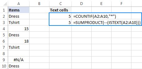
You may also want to look at how to count non-empty cells in Excel.
Count if cell contains specific text
To count cells that contain specific text, use a simple COUNTIF formula like shown below, where range is the cells to check and text is the text string to search for or a reference to the cell containing the text string.
For example, to count cells in the range A2:A10 that contain the word "dress", use this formula:
=COUNTIF(A2:A10, "dress")
Or the one shown in the screenshot:

You can find more formulas examples here: How to count cells with text in Excel: any, specific, filtered cells.
Count if cell contains text (partial match)
To count cells that contain a certain substring, use the COUNTIF function with the asterisk wildcard character (*).
For example, to count how many cells in column A contain "dress" as part of their contents, use this formula:
=COUNTIF(A2:A10,"*dress*")
Or, type the desired text in some cell and concatenate that cell with the wildcard characters:
=COUNTIF(A2:A10,"*"&D1&"*")

For more information, please see: COUNTIF formulas with partial match.
Count if cell contains multiple substrings (AND logic)
To count cells with multiple conditions, use the COUNTIFS function. Excel COUNTIFS can handle up to 127 range/criteria pairs, and only cells that meet all of the specified conditions will be counted.
For example, to find out how many cells in column A contain "dress" AND "blue", use one of the following formulas:
=COUNTIFS(A2:A10,"*dress*", A2:A10,"*blue*")
Or
=COUNTIFS(A2:A10,"*"&D1&"*", A2:A10,"*"&D2&"*")

Count if cell contains number
The formula to count cells with numbers is the simplest formula one could imagine:
Please keep in mind that the COUNT function in Excel counts cells containing any numeric value including numbers, dates and times, because in terms of Excel the last two are also numbers.
In our case, the formula goes as follows:
=COUNT(A2:A10)
To count cells that DO NOT contain numbers, use the SUMPRODUCT function together with ISNUMBER and NOT:
=SUMPRODUCT(--NOT(ISNUMBER(A2:A10)))
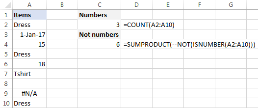
For more examples, see Excel formulas to count cells with certain text.
Sum if cell contains text
If you are looking for an Excel formula to find cells containing specific text and sum the corresponding values in another column, use the SUMIF function.
For example, to find out how many dresses are in stock, use this formula:
=SUMIF(A2:A10,"*dress*",B2:B10)
Where A2:A10 are the text values to check and B2:B10 are the numbers to sum.
Or, put the substring of interest in some cell (E1), and reference that cell in your formula, as shown in the screenshot below:

To sum with multiple criteria, use the SUMIFS function.
For instance, to find out how many blue dresses are available, go with this formula:
=SUMIFS(B2:B10, A2:A10,"*dress*",A2:A10,"*blue*")
Or use this one:
=SUMIFS(B2:B10, A2:A10,"*"&E1&"*",A2:A10,"*"&E2&"*")
Where A2:A10 are the cells to check and B2:B10 are the cells to sum.

Perform different calculations based on cell value
In our last tutorial, we discussed three different formulas to test multiple conditions and return different values depending on the results of those tests. And now, let's see how you can perform different calculations depending on the value in a target cell.
Supposing you have sales numbers in column B and want to calculate bonuses based on those numbers: if a sale is over $300, the bonus is 10%; for sales between $201 and $300 the bonus is 7%; for sales between $101 and $200 the bonus is 5%, and no bonus for under $100 sales.
To have it done, simply multiply the sales (B2) by a corresponding percentage. How do you know which percentage to multiply by? By testing different conditions with nested IFs:
=B2*IF(B2>=300,10%, IF(B2>=200,7%, IF(B2>=100,5%,0)))
In real-life worksheets, it may be more convenient to input percentages in separate cells and reference those cells in your formula:
=B2*IF(B2>=300,$F$5,IF(B2>=200,$F$4,IF(B2>=100,$F$3,$F$2)))
The key thing is fixing the bonus cells' references with the $ sign to prevent them from changing when you copy the formula down the column.

Excel conditional formatting if cell contains specific text
If you want to highlight cells with certain text, set up an Excel conditional formatting rule based on one of the following formulas.
Case-insensitive:
Case-sensitive:
For example, to highlight SKUs that contain the words "dress", make a conditional formatting rule with the below formula and apply it to as many cells in column A as you need beginning with cell A2:
=SEARCH("dress", A2)>0
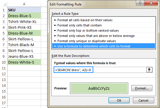
Excel conditional formatting formula: if cell contains text (multiple conditions)
To highlight cells that contain two or more text strings, nest several Search functions within an AND formula. For example, to highlight "blue dress" cells, create a rule based on this formula:
=AND(SEARCH("dress", A2)>0, SEARCH("blue", A2)>0)
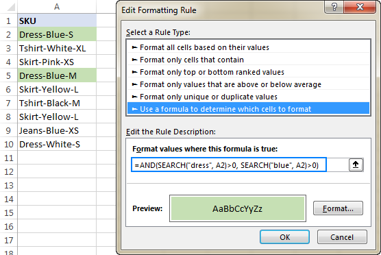
For the detailed steps, please see How to create a conditional formatting rule with a formula.
If cell contains certain text, remove entire row
In case you want to delete rows containing specific text, use Excel's Find and Replace feature in this way:
- Select all cells you want to check.
- Press Ctrl + F to open the Find and Replace dialog box.
- In the Find what box, type the text or number you are looking for, and click the Find All
- Click on any search result, and then press Ctrl + A to select all.
- Click the Close button to close the Find and Replace
- Press Ctrl and the minus button at the same time (Ctrl -), which is the Excel shortcut for Delete.
- In the Delete dialog box, select Entire row, and click OK. Done!
In the screenshot below, we are deleting rows containing "dress":

If cell contains, select or copy entire rows
In situations when you want to select or copy rows with relevant data, use Excel's AutoFilter to filter such rows. After that, press Ctrl + A to select the filtered data, Ctrl+C to copy it, and Ctrl+V to paste the data to another location.
To filter cells with two or more criteria, use Advanced Filter to find such cells, and then copy the entire rows with the results or extract only specific columns.
This is how you manipulate cells based on their value in Excel. I thank you for reading and hope to see you on our blog next week!
Practice workbook
Excel If Cell Contains Then - examples (.xlsx file)
Latest comments
I tried using SUBTOTAL(Function,Range to count). Excel provides you an option to Select the operation (Add/Subtract/Divide etc..) under Function and range of values where you need to count and list in another cell. My requirement was to Sum the value in a range based on filter selected.
Hi! The answer to your question can be found in this article: Excel SUBTOTAL function with formula examples.
Argument Function 101 - 111 ignore all hidden cells - filtered out and hidden manually. For example:
=SUBTOTAL(109,C2:C20)
I have a spreadsheet with quotes, quote amount, PO and then finaly invoice number. I want to calculate on the lines that has a inv number on the quote amount. In other words what has been invoiced.
Hi! To find the total amount for a specific invoice number, you can use the COUNTIF function. If you need to find a sum for more than one condition, use these instructions: How to use Excel COUNTIFS and COUNTIF with multiple criteria.
Hi,
I have a sheet of our business with various branches in our region. I pull a report daily from our ERP system of all the products with stock codes starting with "F" i.e. "Fxxxxxxx"
The branch name is in column A, the Stock codes are in Column B and the sales value of each product is in column E.
I need a formula to extract the total sales value for each branch on stock items with F codes. Can anyone help?
Hi! You can use the SUMIF formula to determine the value of sales for a specific branch. Read more: How to use SUMIF function in Excel with formula examples. Use these instructions if you have multiple conditions to summarize: Excel SUMIFS and SUMIF with multiple criteria. I hope it’ll be helpful. If something is still unclear, please feel free to ask.
Hi! I was wondering if you could help me formulate a cell. I'm trying to formulate a cell so that when the sum of other cells (B2-B10) is equal or less than 14 the word 'low' will populate, and if the sum is equal or greater than 15 the word 'high' will populate.
Thank you so much!
Hi! Calculate the sum of the cells using the SUM function. If these cells contain integers, you can use the IF formula.
=IF(SUM(B2:B10)<=14,"low","high")
If the sum can be a fractional number, try the nested IF formula.
=IF(SUM(B2:B10)<=14,"low",IF(SUM(B2:B10)>=15,"high",""))
Have a sort of complex question about formulas…
G4 – T4 contain numbers. These numbers are serving as a “point value”. G4 is worth 1 “point” so 1 is entered in the cell, M4 is worth 3 “points” so 3 is entered in the cell, etc.
I have names entered into column F (F8 – F40). Each Row contains a different name.
I am attempting to create a matrix where I can enter a date of completion into cells G8:G40 – T8:T40. Once that date is entered, I want to have it add the “points” from each column.
Example:
Bill Kapri has a date of completion entered into cell G10, M10, and R10.
Column G has a “point value” of 1 (number entered into cell G4), Column M has a “point value” of 3 (number entered into cell M4), and Column R has a "point value” of 1 (number entered into cell R4).
I’d like the total of those “points” from row 4 to add together, only for the columns with a date of completion entered.
--
What formula would I need to accomplish such a task? Is this possible?
Hi! If I understand your task correctly, the following formula should work for you:
=SUMPRODUCT(($G$4:$T$4)*(G8:T8<>""))
Read more: Excel SUMPRODUCT function with multiple criteria.
Thank you! Really appreciate your help and the link to additional information.
Hi there,
I found this explanation very useful, but I haven't been able to find the right formula for what I am trying to do yet. I have a table with two columns: one with the name of the month and year in a MMMYY format ('Jan20, 'Feb20, etc.) and another with numbers (=total amount for each month). Is there a formula that would allow me to select/write down two of the first column values and get the sum of all the totals in that range. For example:
Jan20 --- 100
Feb20 --- 250
Mar20 --- 75
Apr20 --- 89
May20 --- 183
In my summary table, writing "Feb20" in one cell (let's say, B3) and "May20" in the next one (C3) would produce a result of "597" in the cell where the formula resides (D3).
Do you think it's doable? Let me know if you need any more details. Thank you!
Hi! If I understand your source data correctly, you have text in the first column, not a date. Therefore, you cannot calculate the sum in the time interval. If the date is written, you can use SUMIF function and this instruction: How to use Excel SUMIF with dates.
Hi.. i need to sum a row of cells with numbers and text but ignore the text. apparently i tried varies formula i cant get the total sum to remain as it will minus the amt when i input a text in one of the row.. pls help
eg. i hv a row for Feb (1 feb - 29 Feb)
in the row below each date, ive input either a OFF or 1
eg. 1 Feb - OFF, 2 Feb - 1, 3 Feb - 1 <- i use =COUNTIF(I80:K80,"1")*2.2 = 4.4
BUT when i insert a text in 2 FEB-RED, it will minus the text and the sub-total number = 2.2
Hi! Your formula only counts cells with 1 in them. It is difficult to understand from your explanation what result you need. Maybe this article will be helpful: COUNTIF function in Excel - count if not blank, greater than, duplicate or unique.
Thank you for this page.
I have a report with 10 columns and 18139 lines. In the B column are product codes (ie RTPGH07304) and the H column has a quantity. The product codes may be repeated several times down the B column. I want to figure out the total quantity overall for a particular product code. For instance, the RTPGH07304 product code may appear three separate times in the B column. In the H column, there is a quantity of 2, 4, and 6 for those separate lines. I want to be able to return a total of 12 to show how many copies of that product were sold. I believe the idea is like the ‘Sum if cell contains text’ section on this page, but I cannot figure it out.
Thank you for your help with this.
Hello! To calculate the total quantity for a specific type of product, use the SUMIF function. For example:
=SUMIF(B$2:B$20000,B2,H$2:H$20000)
You can copy this formula down along the column.
Try to use the recommendations described in this article: How to use SUMIF function in Excel with formula examples. I hope it’ll be helpful.
Hey, I am trying to create a an absenteeism tracker and would like to be able to track the number of Overtime hours - I have row D4 to AH4 with the days of the months - I want to be able to code overtime as OT## and get a sum of the number of OT hours each employee works in AM4 - - Can I total the number beside the code OT in the row?
Hi! To identify cells containing the text 'OT###', use the ISNUMBER and SEARCH functions. The cells containing 'OT###' will have the value 1 in the resulting array. Before performing any mathematical operations, remove 'OT' from these cells using the SUBSTITUTE function. Finally, the two arrays are multiplied and the result is summed.
Try this formula:
=SUM(SUBSTITUTE(D4:AH4,"OT","") * ISNUMBER(SEARCH("OT",D4:AH4)))
I hope this will help.
I have a spreadsheet with multiple tabs. I want to do the following:
Spreadsheet tabs #1 is Detail. This lists the individual prices of each item assigned to a client. Spreadsheet tabs #2 Case and is the summary for each case. I want to take the detailed prices for each client and bring that total of all the detail to the second sheet and have a grand total.
If tab "Detail" has a "Case #" = 44521, then take all the "Extended" prices on that tab and summarize them to the tab "Case" for that specific client
Hi! You can find the sum of all prices for "Case #" using the SUMIF function. But I'm not sure it makes sense to sum the prices. If you want to get all the prices for a specific "Case #", use this guide: Vlookup multiple matches in Excel with one or more criteria. You can also use the FILTER function to get a list of prices. Look for the example formulas here: Excel FILTER function - dynamic filtering with formulas.
It is my hope that my advice will be of help to you in your task.
I want a formula where the cells in a specific range will be counted based on data and criteria in another range.
in the other hand how many cell is in A1:A10 if there is Bi=10,i=1 to 1o
Hi! To count the number of values for a condition, use the COUNTIF function. For example,
=COUNTIF(B1:B10,10)
If there are several such conditions, use the COUNTIFS function.
I am looking to calculate from a spreadsheet, a win-loss record for a team based on the day of the week. If cells a2-a100 represent the day of the week, and cells f2-f100 represent win or loss, how would i write the formula to calculate the winning percentage of all games played on saturday?
Hi! You can calculate the quantity of wins from Saturday using the COUNTIFS formula. I recommend reading this guide: Excel COUNTIFS and COUNTIF with multiple AND / OR criteria. For example:
=COUNTIFS(A2:A100,"Sat",F2:F100,"Win")
Hello,
I have data in column A that has a variety of different variables (ABC, GHY, DUY, IKL, ABC, ABC, DUY, LJK, ABC, IOP, ABC). I have varied dollar amounts in column D that correspond with column A. I want to add all the dollar amounts that are associated with ABC. I have tried but cannot figure this out.
Hi! Use SUMIF function. The following tutorial should help: How to use SUMIF function in Excel with formula examples.
For example,
=SUMIF(A1:A20,"ABC",B1:B20)
I would appreciate any help
I have a spreadsheet with scores from events. Each person has participated in four events and they have four separated scores. I have assigned a point system for scores (i.e a 9 would give someone 20 points). is there a formula(function) that can look at the four cells of scores, determine if they qualify for points assigned and sum them into one cell of total points?
Hello!
To find multiple results that match the condition, use these guidelines and examples: How to Vlookup multiple values in Excel with criteria
If you need to calculate an sum by a condition, use the SUMIF function.
I have read ur example in "Perform different calculations based on cell value". Is there another simple way formula without using IF?
Because i have many tier in "Bonus". it too long if using IF
Hi!
If you have a lot of conditions, use the IFS logic function. Read more in this article: The new Excel IFS function instead of multiple IF.
Hello,
I'm stumped on auto populating a cell. What I want to input is if sheet 2, column A contains any of the same text as sheet 1, column A. Then sheet 2 column 3 will auto populate the same numbers that are showing on Sheet 1, column 3.
Hello!
If I understand your task correctly, the following tutorial should help: VLOOKUP across multiple sheets in Excel with examples.
Need help writing a formula to calculate percentage of invoices validated with payment dates. Essentially, we want to write a formula to generate a count of the cells with dates in them, and to exclude the cells with nothing. Based off this, we are building a gauge chart to depict the percentage of invoices validated. Min value would = 0 and Max value would = total invoices (with & without dates) and this formula would be the main data point showing percentage of invoices ONLY with payment dates tied to them.
Any tips/advice are greatly appreciated!
Hello!
To count the number of cells with dates, try this instruction: Count if blank or not blank. I hope it’ll be helpful. If this is not what you wanted, please describe the problem in more detail.
Hello!
Here is the article that may be helpful to you: Extract number from text string.
Hello,
I'd really appreciate help with a formula.
Column E is an IF statement and depending on a date range puts "YES" or "NO" in column E.
I'm trying to get a separate cell to provide the SUM of the number of "YES"s. SUM and SUMIF do not appear to work. For example, I have attempted the formula =SUMIF(E2:E20,"YES"). It incorrectly provides "0" as the answer. Is this because Column E is a separate formula itself. How do I get around this?
Your help is much appreciated.
Hello!
The SUMIF formula works with the results of formulas in the same way as with normal values. Your formula should work. Check what values are returned by your formulas in cells E2:E20. Perhaps there are extra spaces.
I have an Excel sheet where in column A i have various dates for sales over a three year period and in column B I have another column which contains text relating to the type of sale, either "Direct" or "Indirect" to indicate if the sale was a direct sale or through another party. I want to be able to count how many Direct or Indirect sales were made in each year. Can you help? I have tried combining the COUNTIF and COUNTIFS formulas but it's not working. I can get the number of sales in each year by using the COUNTIFS formula but the problem starts when I try to extract the count in each year for each of Direct or Indirect by combining the two formulas. Thanks! Your website is amazing! I've managed to solve a lot of problems by checking your solutions.
Hello!
What formulas are you using? What's not working in them? You must use the COUNTIFS formula with two conditions - Date and Sales Type.
Please have a look at this article - Excel COUNTIFS and COUNTIF with multiple AND/OR criteria
If they don’t work for you, then please describe your task in detail, I’ll try to suggest a solution.