In our previous tutorial, we were looking at Excel If contains formulas that return some value to another column if a target cell contains a given value. Aside from that, what else can you do if a cell contains specific text or number? A variety of things such as counting or summing cells, highlighting, removing or copying entire rows, and more.
Excel 'Count if cell contains' formula examples
In Microsoft Excel, there are two functions to count cells based on their values, COUNTIF and COUNTIFS. These functions cover most, though not all, scenarios. The below examples will teach you how to choose an appropriate Count if cell contains formula for your particular task.
Count if cell contains any text
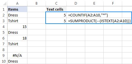
In situations when you want to count cells containing any text, use the asterisk wildcard character as the criteria in your COUNTIF formula:
Or, use the SUMPRODUCT function in combination with ISTEXT:
In the second formula, the ISTEXT function evaluates each cell in the specified range and returns an array of TRUE (text) and FALSE (not text) values; the double unary operator (--) coerces TRUE and FALSE into 1's and 0's; and SUMPRODUCT adds up the numbers.
As shown in the screenshot below, both formulas yield the same result:
=COUNTIF(A2:A10,"*")
=SUMPRODUCT(--(ISTEXT(A2:A10)))

You may also want to look at how to count non-empty cells in Excel.
Count if cell contains specific text
To count cells that contain specific text, use a simple COUNTIF formula like shown below, where range is the cells to check and text is the text string to search for or a reference to the cell containing the text string.
For example, to count cells in the range A2:A10 that contain the word "dress", use this formula:
=COUNTIF(A2:A10, "dress")
Or the one shown in the screenshot:

You can find more formulas examples here: How to count cells with text in Excel: any, specific, filtered cells.
Count if cell contains text (partial match)
To count cells that contain a certain substring, use the COUNTIF function with the asterisk wildcard character (*).
For example, to count how many cells in column A contain "dress" as part of their contents, use this formula:
=COUNTIF(A2:A10,"*dress*")
Or, type the desired text in some cell and concatenate that cell with the wildcard characters:
=COUNTIF(A2:A10,"*"&D1&"*")

For more information, please see: COUNTIF formulas with partial match.
Count if cell contains multiple substrings (AND logic)
To count cells with multiple conditions, use the COUNTIFS function. Excel COUNTIFS can handle up to 127 range/criteria pairs, and only cells that meet all of the specified conditions will be counted.
For example, to find out how many cells in column A contain "dress" AND "blue", use one of the following formulas:
=COUNTIFS(A2:A10,"*dress*", A2:A10,"*blue*")
Or
=COUNTIFS(A2:A10,"*"&D1&"*", A2:A10,"*"&D2&"*")

Count if cell contains number
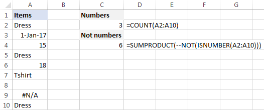
The formula to count cells with numbers is the simplest formula one could imagine:
Please keep in mind that the COUNT function in Excel counts cells containing any numeric value including numbers, dates and times, because in terms of Excel the last two are also numbers.
In our case, the formula goes as follows:
=COUNT(A2:A10)
To count cells that DO NOT contain numbers, use the SUMPRODUCT function together with ISNUMBER and NOT:
=SUMPRODUCT(--NOT(ISNUMBER(A2:A10)))

For more examples, see Excel formulas to count cells with certain text.
Sum if cell contains text
If you are looking for an Excel formula to find cells containing specific text and sum the corresponding values in another column, use the SUMIF function.
For example, to find out how many dresses are in stock, use this formula:
=SUMIF(A2:A10,"*dress*",B2:B10)
Where A2:A10 are the text values to check and B2:B10 are the numbers to sum.
Or, put the substring of interest in some cell (E1), and reference that cell in your formula, as shown in the screenshot below:

To sum with multiple criteria, use the SUMIFS function.
For instance, to find out how many blue dresses are available, go with this formula:
=SUMIFS(B2:B10, A2:A10,"*dress*",A2:A10,"*blue*")
Or use this one:
=SUMIFS(B2:B10, A2:A10,"*"&E1&"*",A2:A10,"*"&E2&"*")
Where A2:A10 are the cells to check and B2:B10 are the cells to sum.

Perform different calculations based on cell value
In our last tutorial, we discussed three different formulas to test multiple conditions and return different values depending on the results of those tests. And now, let's see how you can perform different calculations depending on the value in a target cell.
Supposing you have sales numbers in column B and want to calculate bonuses based on those numbers: if a sale is over $300, the bonus is 10%; for sales between $201 and $300 the bonus is 7%; for sales between $101 and $200 the bonus is 5%, and no bonus for under $100 sales.
To have it done, simply multiply the sales (B2) by a corresponding percentage. How do you know which percentage to multiply by? By testing different conditions with nested IFs:
=B2*IF(B2>=300,10%, IF(B2>=200,7%, IF(B2>=100,5%,0)))
In real-life worksheets, it may be more convenient to input percentages in separate cells and reference those cells in your formula:
=B2*IF(B2>=300,$F$5,IF(B2>=200,$F$4,IF(B2>=100,$F$3,$F$2)))
The key thing is fixing the bonus cells' references with the $ sign to prevent them from changing when you copy the formula down the column.

Excel conditional formatting if cell contains specific text
If you want to highlight cells with certain text, set up an Excel conditional formatting rule based on one of the following formulas.
Case-insensitive:
Case-sensitive:
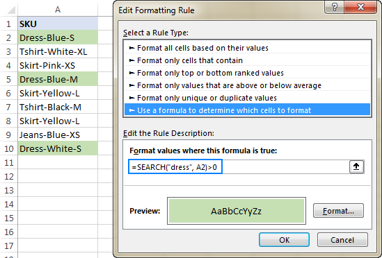
For example, to highlight SKUs that contain the words "dress", make a conditional formatting rule with the below formula and apply it to as many cells in column A as you need beginning with cell A2:
=SEARCH("dress", A2)>0

Excel conditional formatting formula: if cell contains text (multiple conditions)
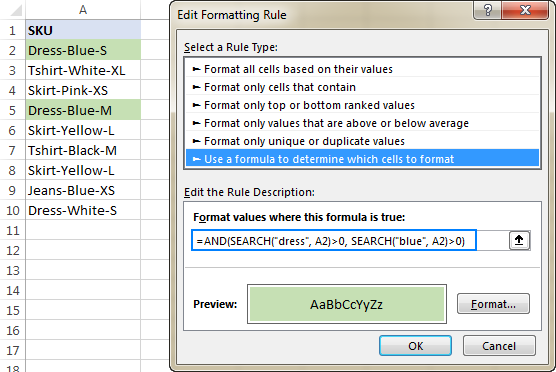
To highlight cells that contain two or more text strings, nest several Search functions within an AND formula. For example, to highlight "blue dress" cells, create a rule based on this formula:
=AND(SEARCH("dress", A2)>0, SEARCH("blue", A2)>0)

For the detailed steps, please see How to create a conditional formatting rule with a formula.
If cell contains certain text, remove entire row
In case you want to delete rows containing specific text, use Excel's Find and Replace feature in this way:
- Select all cells you want to check.
- Press Ctrl + F to open the Find and Replace dialog box.
- In the Find what box, type the text or number you are looking for, and click the Find All
- Click on any search result, and then press Ctrl + A to select all.
- Click the Close button to close the Find and Replace
- Press Ctrl and the minus button at the same time (Ctrl -), which is the Excel shortcut for Delete.
- In the Delete dialog box, select Entire row, and click OK. Done!
In the screenshot below, we are deleting rows containing "dress":

If cell contains, select or copy entire rows
In situations when you want to select or copy rows with relevant data, use Excel's AutoFilter to filter such rows. After that, press Ctrl + A to select the filtered data, Ctrl+C to copy it, and Ctrl+V to paste the data to another location.
To filter cells with two or more criteria, use Advanced Filter to find such cells, and then copy the entire rows with the results or extract only specific columns.
This is how you manipulate cells based on their value in Excel. I thank you for reading and hope to see you on our blog next week!
Practice workbook
Excel If Cell Contains Then - examples (.xlsx file)
 by
by
244 comments
I need help with this formula. =SUMIF($D:$D,"*Wave 1*",$F:$F)
Right now I want to add values from F if D says Wave 1 however if the the sum is 0 i want it to say TBD .. not sure how to do the TBD part
Hi!
What is TBD? Please describe your problem in more detail.
Hi,
I need to add values in alternative cells. eg: values in I5,K5,M5 and the sum should ignore text in those cells. Please suggest
In fact i would like to know whether excel can display the value of a cell in another cell by using an IF condition.
e.g value of A1 is "FLOWERS"
input text "FL" in B1
the result should be the value of A1 to be displayed in C1 if you put a condition that if the value of B1 = "FL"
is there any formula to solve this.
thanks
Hello!
You can learn more about IF function in Excel in this article on our blog.
IF(B1="FL",A1,"")
I have a list of parts in column A, then i have a list of dates in column B
I want the formula to return how many times each part number has a date beside it
123456 1-jan-21
234567 5-jan-21
123456
123456 5-feb-21
so i would want this to return
123456 2
234567 1
Hello!
If I got you right, the formula below will help you with your task:
=COUNTIFS(A1:A100,D1,B1:B100," < > "&"")
D1="123456"
You can learn more about COUNTIFS function in Excel in this article on our blog
I hope it’ll be helpful.
Please help me figure this out. I have a spreadsheet of pupils' scores on a test. I have put a '1' in a cell if they got the question correct, a '0' if incorrect and a '.' if they didn't attempt it. I have a separate list to the side which says the name of the topic next to each question number. I would like to generate a list of topics they need to practice for each pupil based on the questions they got wrong. How can I do this? For example, if they got question 8 and 10 incorrect and these questions were a multiplication and a division question I would like a list which says multiplication and division. Please help me figure this out!
Hello!
Please use the following array formula -
{=IFERROR(INDEX($C$3:$C$30, SMALL(IF(1=((--($I3=$A$3:$A$30))*(--($J3=$B$3:$B$30))), ROW($C$3:$C$30)-2,""), COLUMN()-10)),"")}
A3:C30 - your table, I3 - name, J3 - zero or "." K3 - this formula.
Please have a look at this article - Vlookup multiple matches and return results in a row (Formula 2)
I hope I answered your question. If something is still unclear, please feel free to ask.
Hi Everyone, I would really like some help with this logic
I would like to create a formula in cell C2, if D2 = text "X" perform sum of A2 + B2, but if D2 = text "W" cell = just the value in B2
I hope this makes sense, TIA
Hi,
Please have a look at this article: Nested IF in Excel – formula with multiple conditions
It contains answers to your question
If all my cells contains value,(without blank) then I should get the output as T else F
Will anyone please help me out
What I'm looking for is a formula that will do the following:
If cell a1 contains specific text, then count cell a2.
I've tried all sorts of different options, but can't get it to show the right count.
Hello!
You can check the text written in the cell using the ISTEXT function. Use it in an IF function statement. I don't quite understand what "count cell a2" means.
Here is an example of what I've attempting. Perhaps this might help.
If in the range of data, X appears, then count the next cell after X (which would have A, B, or C in it).
Thank you for all the Information they are great. what i would like to dois:
I Have in column A a data validation that has X,Y Z and on a different sheet under X i have a list of names in a column as well as under Y ans Z. what I want, is when I choose for example X in column A, I want in column B automatically to copy all the names of the other sheet under X into the cells in column B into a column not row? please can you help me with this problem?
Hello, could you please help me to find formula that highlights the cell with specific text when the text is a list? Is this the correct way to do it in Conditional Formatting (by formula)?
=ISNUMBER(MATCH($A$2,List,0))
when list is the range of list cells?
If this is the best way, Is there a way to copy this exact formatting to other cells (format painter doesn't do the job)?
Thank you so much in advance.
Hello Ludmila!
If I understand your task correctly, the following conditional formatting formula should work for you:
=ISNUMBER(MATCH($A$2,F2,0))
where F2 is the first cell of the list cell range.
I hope it’ll be helpful.
Hello Alexander, thank you for your answer. Unfortunately, the formula you've suggested didn't work for me, though the formula that includes range of cells containing the list works well.
My additional question was is there a way to apply the same conditional formatting formula to multiple cells. I mean is there a fast way to copy the conditional formatting formula that will be updated to other cells (eg A3, A4 and so on) instead of creating a new rule for every next cell? Thank you!
Hello!
I'm sorry the formula wasn't useful to you. Apparently, we represent your data differently.
How to copy conditional formatting is described here.
I am looking to use a condition on one cell (A2=Kabul, then pick data from another sheet, K5) and the same condition will be repeated in one formula (A2=Laghman, A2=Logar..... and then data will be picked from a different cell). How I can do it?
Hello Ebadullah!
I’m sorry but your task is not entirely clear to me.
For me to be able to help you better, please describe your task in more detail. Please let me know in more detail what you were trying to find, what formula you used and what problem or error occurred. Give an example of the source data and the expected result. It’ll help me understand it better and find a solution for you. Thank you.
Hi there,
How do I Sum out multiple SKUs when I keyed them in according to the warehouse racking layout?
Example :
A1 B1 C1 are the name of the SKUs, while A1 C1 has the same SKU.
A2 B2 C2 will be the Quantity of each SKU above.
How do I get the the sum of A2 and C2 in a separate list if we got 600 SKUs.
Thank you.
Please if cell b4 has a data of 24pcs and cell c4 has 34000....
I want to multiply the two cell together...
Please how can I go about this.
Thanks
Hello Gbenga!
If I understand your task correctly, the following formula should work for you
=LEFT(A1,LEN(A1) - FIND("pcs",A1)) * B1
Hope you’ll find this information helpful.
Hello George!
In order to extract all the characters after "UL9", use the formula below:
=RIGHT(A10, LEN(A1) - FIND("UL9", A1,1) +1)
As for pulling the text before "UL9", here is the formula for this case:
=LEFT(A1, FIND("UL9", A1 ,1) - 1)
BTW, there is a formula-free solution for this task called Extract Text tool. Check out its manual, I believe you'll find it helpful: https://www.ablebits.com/docs/excel-extract-text/
How can I delete upon scanning a bar code, everything except the text that starts with UL9C0037365 value in a cell
01008568230065341119071521UL9C0037365
Thank you
george
Thank you so much for most helpful forumula
How do I have a cell calculate a sum if there's a certain word or text in another cell? I.E. 12345*2% will only be calculated if say cell A5 was showing the word "No".
Thanks!
I need a formula that will search a specific cell (E2) or all of column E for a "key" word and then if found, take the date in A2 and add 30 days to it and put this all in B2.
Please let me know if this can be accomplished.
Thanks.
Hello,
Did you find a solution for your issue? I am currently trying to find something similar. I need to find all people who are online and add their hours, ignoring those who are on leave etc, Can anyone help?
Thanks in advance
Hi,
Is there a solution for this?
Basically, I have month in one column and dollars in another. If I want the sum of all the dollars in June, July and Aaugust in a separate column. Is there a formula that does this. I am sure there is but cannot figure it out.
Thanks,
Dinesh.
Month dollar sum
June 20
June 30
June 25
June 22
June 31 sum of June dollars
July 18
July 16
July 15
July 22
July 19 sum of July dollars
August 6
August 3
August 32
August 34
August 24 sum of Aug dollars
Any Help Apprecaiated:
Essentially I am trying to write a formula where if all cells in a column range contain a numerical value it will SUM them, but add a condition where if the column contains a text it will search for the text and instead of returning a SUM it will return "Not Complete".
Currently I am working with the following formula but cant seem to get it to work:
=IF(ISNUMBER(SEARCH("Not Complete",H4:$H2000)),"Not Complete",SUM(H4:$H2000))
For Reference:
Column of values mixed with text containing "Not Complete"
$0.052000
$0.052000
$0.052000
$0.052000
Not Complete
Not Complete
Not Complete
Not Complete
$0.052000
$0.052000
$0.052000