The tutorial looks at how to use the ISTEXT and ISNONTEXT functions in Excel to check if a cell contains a textual value or not.
Whenever you need to get information about the contents of some cell in Excel, you'd typically use the so-called Information functions. Both ISTEXT and ISNONTEXT belong to this category. The ISTEXT function checks if a value is text and ISNONTEXT tests if a value is not text. Whatever simple the concept is, the functions are amazingly useful for solving a variety of different tasks in Excel.
Excel ISTEXT function
The ISTEXT function in Excel checks is a specified value is text or not. If the value is textual, the function returns TRUE. For all other data types (such as numbers, dates, blank cells, errors, etc.) it returns FALSE.
The syntax is as follows:
ISTEXT(value)
Where value is a value, cell reference, expression or another function whose result you want to test.
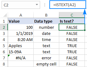
For example, to find out whether a value in A2 is text or not, use this simple formula:
=ISTEXT(A2)
Excel ISNONTEXT function
The ISNONTEXT function returns TRUE for any non-text value including numbers, dates and times, blanks, and other formulas that return non-textual results or errors. For text values, it returns FALSE.
The syntax is the same as that of the ISTEXT function:
ISTEXT(value)
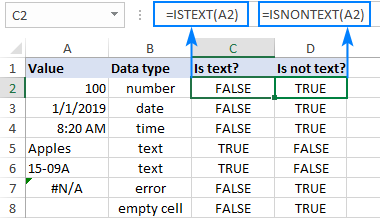
For instance, to check if a value in A2 is not text, use this formula:
=ISNONTEXT(A2)
As shown in the screenshot below, the ISTEXT and ISNONTEXT formulas return the opposite results:
ISTEXT and ISNONTEXT functions in Excel - usage notes
ISTEXT and ISNONTEXT are very straightforward and easy-to-use functions, and you are unlikely to run into any difficulties with them. That said, there are a few keys points to take notice of:
- Both functions are part of the IS functions group that return the logical (Boolean) values of TRUE or FALSE.
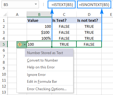
- In a specific case when numbers are stored as text, ISTEXT returns TRUE and ISNONTEXT returns FALSE.
- Both functions are available in all versions of Excel for Office 365, Excel 2019, Excel 2016, Excel 2013, Excel 2010, Excel 2007, Excel 2003, Excel XP, and Excel 2000.
Using ISTEXT and ISNONTEXT in Excel - formula examples
Below you will find examples of practical uses of the ISTEXT and ISNONTEXT functions in Excel that will hopefully help you make your worksheets more efficient.
Check if a value is text
Sometimes when you are working with a bunch of values, you may be surprised to notice that for some numbers your formulas return wrong results or even errors. The most obvious reason is that problematic numbers are stored as text. The below formulas will tell you for sure which values are text from Excel's viewpoint.
ISTEXT formula:
Returns TRUE for any value that Excel considers text.
=ISTEXT(B2)
ISNONTEXT formula:
Returns TRUE for any value that Excel considers non-text.
=ISNONTEXT(B2)
ISTEXT for Data Validation: allow text only
In some situations, you may want to allow users to enter only text values in certain cells. To achieve this, create a data validation rule based on an ISTEXT formula. Here's how:
- Select one or more cells that you want to validate.
- On the Data tab, in the Data Tools group, click the Data Validation button.
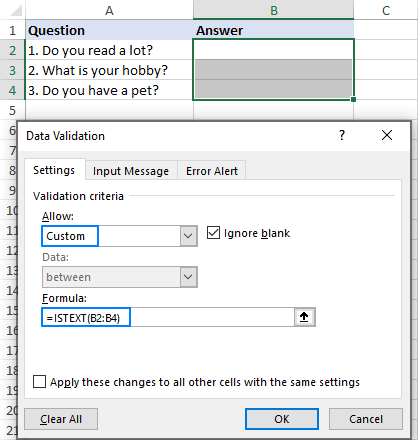
- On the Settings tab of the Data Validation dialog box, select Custom for the validation criteria and enter your ISTEXT formula in the corresponding box.
- Click OK to save the rule.
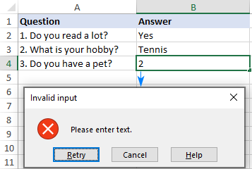
For this example, we are validating the questionnaire answers in cells B2 through B4 with the help of this formula:
=ISTEXT(B2:B4)
Additionally, you can configure your own Error Alert message to explain to your users what kind of data is accepted:
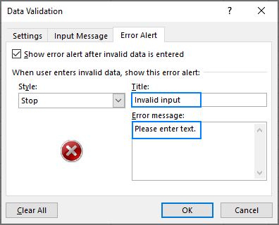
As the result, when the user tries to enter a number or date in any of the validated cells, they will see the following alert:
For more information, please see Using Data validation in Excel.
Excel IF ISTEXT formula
In practice, ISTEXT and ISNONTEXT are often used together with the IF function to output a more user friendly result than the standard TRUE and FALSE.
Formula 1. If is text, then
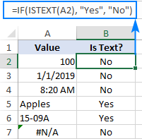
Taking our very first example a little further, supposing you want to return "Yes" for text values and "No" for anything else. To have it done, simply nest the ISTEXT function into the logical test of IF, and use "Yes" and "No" for the value_if_true and value_if_false arguments, respectively:
=IF(ISTEXT(A2), "Yes", "No")
Formula 2. Check cell's input
In one of the previous examples, we discussed how to ensure valid user input by using Data Validation. This can also be done in a "milder" form with the help of an Excel IF ISTEXT formula.
In the questionnaire, suppose you want to determine which answers are valid (text) and which are not (non-text). For this, use the nested IF statements with the following logic:
- If the tested cell is empty, return nothing, i.e. an empty string ("").
- If the cell is text, return "Valid answer".
- If neither of the above, return "Invalid answer - please enter text."
Putting all this together, we get the following formula, where B2 is the cell to be checked:
=IF(B2="", "", IF(ISTEXT(B2), "Valid answer", "Invalid answer - please enter text."))

Check if a range contains any text
So far, we have tested each cell individually. But what if you need to know whether any cell in a range contains text?
To test the entire range, combine the ISTEXT function with SUMPRODUCT in this way:
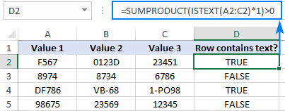
As an example, let's check each row in the below data set for text values, which can be done with the following formulas:
=SUMPRODUCT(ISTEXT(A2:C2)*1)>0
=SUMPRODUCT(--ISTEXT(A2:C2))>0
One of the above formulas goes to cell D2, and then you drag it down through cell D5.
So, you now have a clear understanding which rows contain one or more text strings (TRUE) and which contain only numbers (FALSE).
If you'd like to return different results, say "Yes" or "No" as opposed to TRUE and FALSE, enclose the above formula in the IF statement:
=IF(SUMPRODUCT(--ISTEXT(A2:C2))>0, "Yes", "No")
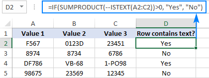
How this formula works
The formula is based on the ability of SUMPRODUCT to handle arrays natively. Working from the inside out, here's what it does:
- The ISTEXT function returns an array of TRUE and FALSE values. For A2:C2, we get this array:
{TRUE,TRUE,FALSE} - Next, we multiple each element of the above array by 1 to convert the logical values of TRUE and FALSE into 1's and 0's, respectively. A double unary operator (--) can be used for the same purpose. After the transformation, the formula takes this form:
SUMPRODUCT({1,1,0})>0 - The SUMPRODUCT function adds up 1's and 0's, and you check if the result is greater than zero. If it is, the range contains at least one text value and the formula returns TRUE, if not FALSE.
Check if a cell contains specific text
The Excel ISTEXT function can only determine whether a cell contains text, meaning absolutely any text. To find out whether a cell contains a specific text string, use either the ISNUMBER SEARCH formula or COUNTIF with wildcards.
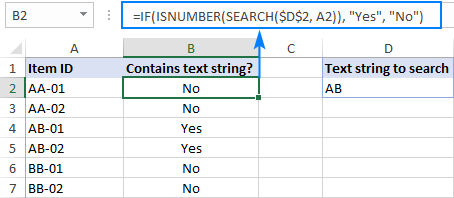
For example, to see if the Item Id in A2 contains the text string input in cell D2, use the below formula (please mind the absolute reference $D$2 that prevents the cell address from changing when the formula is copied to other cells):
=ISNUMBER(SEARCH($D$2, A2))
For the sake for convenience, we'll wrap it into the IF function:
=IF(ISNUMBER(SEARCH($D$2, A2)), "Yes", "No")
And get the following results:
The same result can be achieved with COUNTIF:
=IF(COUNTIF(A2, "*"&$D$2&"*")>0, "Yes", "No")

For more examples, please see Excel If cell contains formulas.
Highlight cells that contain text
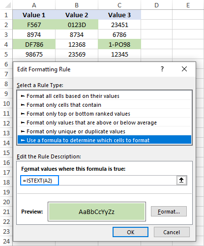
The ISTEXT function can also be used with Excel conditional formatting to highlight cells containing text values. Here's how:
- Select all the cells that you want to check and highlight (A2:C5 in this example).
- On the Home tab, in the Styles group, click New Rule > Use a formula to determine which cells to format.
- In the Format values where this formula is true box, enter the below formula:
=ISTEXT(A2)Where A2 is the leftmost cell of the selected range.
- Click the Format button and choose the desired formatting.
- Click OK twice to close both dialog boxes and save the rule.
For more detailed explanation of each step, please see: Using formulas for Excel conditional formatting.
As the result, Excel highlights all the cells with any text strings:
That's how to use the ISTEXT and ISNONTEXT functions in Excel. I thank you for reading and hope to see you on our blog next week!
 by
by
7 comments
In A1 I have "Peter"
In A2 I have =IF (A1="Peter", "", "not Peter") // Result A2 must be ""
In A3 I put Istext(A2) and the result is true even if A2 is "" (Blank) !!! I don't understand
Or ISTEXT is considering the formula in A2 as text ?
Hi! Your formula returns a text value in cell A2. This value contains 0 characters. Therefore, the ISTEXT function returns TRUE.
Your solution for the topic "ISTEXT for Data Validation: allow text only" would not work. Correct me if I'm wrong here. If you select all three cells as you've shown in the screenshot, and then apply the recommended formula "=IsText(B2:B4)", excel will apply that for B2, and automatically apply "=IsText(B3:B5)" for B3 and automatically apply "=IsText(B4:B6)" for B3. Eventually it would not work if you enter any non-text in B5 or B6, a range which is out of the scope of our focus and will create problems.
Correct solution is to apply the formula "=IsText(B2)" and excel will automatically update and apply the formula for B3 and B4. You can even check by going to each cell and pressing Data Validation to check the formula.
Hi! I have not been able to replicate your problem. I have this data validation formula working correctly.
Typo in line 3 - 8th word is B4 (Not B3)
Good article. I want a merged dependent range of cells to check for text within merged precedent cells on another sheet. If text is there, I want the dependent merged cells to display that text. If not, then I want it to display the text from merged cells on another sheet. such as:
=IF(ISTEXT('DETAIL - LUMP SUM'!C12:H12),'DETAIL - LUMP SUM'!C12:H12,'DETAIL - UNIT PRICING'!D12: H12)
When entered, the dependent cells simply display the formula text directly. Any thoughts?
Hi!
I can't check the formula that contains unique references to your workbook worksheets.
The formula IF(ISTEXT(C12:H12),1,0) is equivalent to the formula IF(ISTEXT(C12),1,0). The IF function only works on the first value of the array. To display the values of multiple cells, I recommend concatenating them using the CONCAT function.
The formula might look like this:
=IF(SUM(--ISTEXT(C12:H12)),CONCAT(C12:H12),CONCAT(D12:H12))