 by
by How do I count cells with text in Excel? There are a few different formulas to count cells that contain any text, specific characters or only filtered cells. All the formulas work in Excel 365, 2021, 2019, 2016, 2013 and 2010.
Initially, Excel spreadsheets were designed to work with numbers. But these days we often use them to store and manipulate text too. Want to know how many cells with text there are in your worksheet? Microsoft Excel has several functions for this. Which one should you use? Well, it depends on the situation. In this tutorial, you will find a variety of formulas and when each formula is best to be used.
How to count number of cells with text in Excel
There are two basic formulas to find how many cells in a given range contain any text string or character.
COUNTIF formula to count all cells with text
When you wish to find the number of cells with text in Excel, the COUNTIF function with an asterisk in the criteria argument is the best and easiest solution:
Because the asterisk (*) is a wildcard that matches any sequence of characters, the formula counts all cells that contain any text.
SUMPRODUCT formula to count cells with any text
Another way to get the number of cells containing text is to combine the SUMPRODUCT and ISTEXT functions:
Or
The ISTEXT function checks if each cell in the specified range contains any text characters and returns an array of TRUE (cells with text) and FALSE (other cells) values. The double unary (--) or the multiplication operation coerces TRUE and FALSE into 1 and 0, respectively, producing an array of ones and zeros. The SUMPRODUCT function sums all the elements of the array and returns the number of 1's, which is the number of cells that contain text.
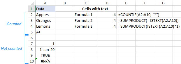
To gain more understanding of how these formulas work, please see which values are counted and which are not:
| What is counted | What is not counted |
|
|
For example, to count cells with text in the range A2:A10, excluding numbers, dates, logical values, errors and blank cells, use one of these formulas:
=COUNTIF(A2:A10, "*")
=SUMPRODUCT(--ISTEXT(A2:A10))
=SUMPRODUCT(ISTEXT(A2:A10)*1)
The screenshot below shows the result:
Count cells with text excluding spaces and empty strings
The formulas discussed above count all cells that have any text characters in them. In some situations, however, that might be confusing because certain cells may only look empty but, in fact, contain characters invisible to the human eye such as empty strings, apostrophes, spaces, line breaks, etc. As a result, a visually blank cell gets counted by the formula causing a user to pull out their hair trying to figure out why :)
To exclude "false positive" blank cells from the count, use the COUNTIFS function with the "excluded" character in the second criterion.
For example, to count cells with text in the range A2:A7 ignoring those that contain a space character, use this formula:
=COUNTIFS(A2:A7,"*", A2:A7, "<> ")
Notice the space character before the closing quote in the second condition ("<> "). The expression reads "not equal to space".

If your target range contains any formula-driven data, some of the formulas may result in an empty string (""). To ignore cells with empty strings too, replace "*" with "*?*" in the criteria1 argument:
=COUNTIFS(A2:A9,"*?*", A2:A9, "<> ")
A question mark surrounded by asterisks indicates that there should be at least one text character in the cell. Since an empty string has no characters in it, it does not meet the criteria and is not counted. Blank cells that begin with an apostrophe (') are not counted either.
In the screenshot below, there is a space in A7, an apostrophe in A8 and an empty string (="") in A9. Our formula leaves out all those cells and returns a text-cells count of 3:

How to count cells with certain text in Excel
To get the number of cells that contain certain text or character, you simply supply that text in the criteria argument of the COUNTIF function. The below examples explain the nuances.
To match the sample text exactly, enter the full text enclosed in quotation marks:
To count cells with partial match, place the text between two asterisks, which represent any number of characters before and after the text:
For example, to find how many cells in the range A2:A7 contain exactly the word "bananas", use this formula:
=COUNTIF(A2:A7, "bananas")
To count all cells that contain "bananas" as part of their contents in any position, use this one:
=COUNTIF(A2:A7, "*bananas*")
To make the formula more user-friendly, you can place the criteria in a predefined cell, say D2, and put the cell reference in the second argument:
=COUNTIF(A2:A7, D2)
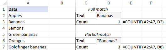
Depending on the input in D2, the formula can match the sample text fully or partially:
- For full match, type the whole word or phrase as it appears in the source table, e.g. Bananas.
- For partial match, type the sample text surrounded by the wildcard characters, like *Bananas*.
As the formula is case-insensitive, you may not bother about the letter case, meaning that *bananas* will do as well.
Alternatively, to count cells with partial match, concatenate the cell reference and wildcard characters like:
=COUNTIF(A2:A7, "*"&D2&"*")

For more information, please see How to count cells with specific text in Excel.
How to count filtered cells with text in Excel
When using Excel filter to display only the data relevant at a given moment, you may sometimes need to count visible cells with text. Regrettably, there is no one-click solution for this task, but the below example will comfortably walk you through the steps.
Supposing, you have a table like shown in the image below. Some entries were pulled from a larger database using formulas, and various errors occurred along the way. You are looking to find the total number of items in column A. With all the rows visible, the COUNTIF formula that we've used for counting cells with text works a treat:
=COUNTIF(A2:A10, "*")
And now, you narrow down the list by some criteria, say filter out the items with quantity greater than 10. The question is – how many items remained?

To count filtered cells with text, this is what you need to do:
- In your source table, make all the rows visible. For this, clear all filters and unhide hidden rows.
- Add a helper column with the SUBTOTAL formula that indicates if a row is filtered or not.
To handle filtered cells, use 3 for the function_num argument:=SUBTOTAL(3, A2)To identify all hidden cells, filtered out and hidden manually, put 103 in function_num:
=SUBTOTAL(103, A2)In this example, we want to count only visible cells with text regardless of how other cells were hidden, so we enter the second formula in A2 and copy it down to A10.
For visible cells, the formula returns 1. As soon as you filter out or manually hide some rows, the formula will return 0 for them. (You won't see those zeros because they are returned for hidden rows. To make sure it works this way, just copy the contents of a hidden cell with the Subtotal formula to any visible say, say =D2, assuming row 2 is hidden.)

- Use the COUNTIFS function with two different criteria_range/criteria pairs to count visible cells with text:
- Criteria1 - searches for cells with any text ("*") in the range A2:A10.
- Criteria2 - searches for 1 in the range D2:D10 to detect visible cells.
=COUNTIFS(A2:A10, "*", D2:D10, 1)
Now, you can filter the data the way you want, and the formula will tell you how many filtered cells in column A contain text (3 in our case):

If you'd rather not insert an additional column in your worksheet, then you will need a longer formula to accomplish the task. Just choose the one you like better:
=SUMPRODUCT(SUBTOTAL(103, INDIRECT("A"&ROW(A2:A10))), --(ISTEXT(A2:A10)))
=SUMPRODUCT(SUBTOTAL(103, OFFSET(A2:A10, ROW(A2:A10) - MIN(ROW(A2:A10)),,1)), -- (ISTEXT(A2:A10)))
The multiplication operator will work as well:
=SUMPRODUCT(SUBTOTAL(103, INDIRECT("A"&ROW(A2:A10))) * (ISTEXT(A2:A10)))
=SUMPRODUCT(SUBTOTAL(103, OFFSET(A2:A10, ROW(A2:A10)-MIN(ROW(A2:A10)),,1)) * (ISTEXT(A2:A10)))
Which formula to use is a matter of your personal preference - the result will be the same in any case:

How these formulas work
The first formula employs the INDIRECT function to "feed" the individual references of all cells in the specified range to SUBTOTAL. The second formula uses a combination of the OFFSET, ROW and MIN functions for the same purpose.
The SUBTOTAL function returns an array of 1's and 0's where ones represent visible cells and zeros match hidden cells (like the helper column above).
The ISTEXT function checks each cell in A2:A10 and returns TRUE if a cell contains text, FALSE otherwise. The double unary operator (--) coerces the TRUE and FALSE values into 1's and 0's. At this point, the formula looks as follows:
=SUMPRODUCT({0;1;1;1;0;1;1;0;0}, {1;1;1;0;1;1;0;1;1})
The SUMPRODUCT function first multiplies the elements of both arrays in the same positions and then sums the resulting array.
As multiplying by zero gives zero, only the cells represented by 1 in both arrays have 1 in the final array.
=SUMPRODUCT({0;1;1;0;0;1;0;0;0})
And the number of 1's in the above array is the number of visible cells that contain text.
That's how to how to count cells with text in Excel. I thank you for reading and hope to see you on our blog next week!
Latest comments
I have 2 columns A and B. In A I have many types of text "Apple", "Banana", "Orange", "Pineapple", "Strawberries. In column B I'm adding the amount for each type of text. In column C I need a formula where when I type only Apple or Banana (Orange, Pineapple, Strawberries - are not important) their amount to be shown in column C.
Thank You
Hi! To get a value by condition, you can use one of these methods: Excel VLOOKUP function tutorial with formula examples or Excel INDEX MATCH vs. VLOOKUP - formula examples or XLOOKUP function in Excel. Choose the method that works best for you.
Can you please help me to:(My data range contains numbers, text and also numbers with formulas and text with formulas
Find out the count of numbers without formula in the data range
Find out the count of text without formula in the data range
Hi! Use the NOT and ISFORMULA functions to identify cells that do not contain formulas. Use the ISNUMBER function to define cells with numbers. Use NOT and ISNUMBER function to identify cells with text. Use the SUMPRODUCT function to find the number of cells you need. For example:
=SUMPRODUCT((NOT(ISFORMULA(A1:A5))) * ISNUMBER(A1:A5))
Excellent Sir, My problem resolved
I have a table in Excel with thousands of rows. If I apply certain filters to any column, the quantity is reduced specifically to the quantity that the filter applies to it. I want to know, how can I make the program count the number of rows and show the result every time I change the filter?
Hello! To count only the visible cells in an Excel range and ignore hidden ones (such as those filtered out), you can use different methods:
1. Using the SUBTOTAL Function:
Enter the formula =SUBTOTAL(3, A1:A100) (where range represents the area you want to count, excluding hidden rows or columns).
2. Using the AGGREGATE Function:
Enter the formula =AGGREGATE(3,5,A1:A100) (where range is the area you want to count, ignoring hidden cells).
Other Excel functions cannot ignore hidden cells.
I want to count (and display) the number of cells in a column that contain text. I am using this formula in cell D24: =COUNTIF(D4:D23,"*")
The sum does not appear in cell D24, but the formula does. What am I doing wrong?
Hi! The answer to your question can be found in this guide: Excel COUNTIF for blank and non-blank cells.
Hi
I am trying to work on 4 columns.
Column D - Year groups ie Year 10, Year 11, Year 12
Column J - 1st colour ie red, green, blue
Column K - 2nd colour ie red, green, blue
Column L - 3rd colour ie red, green, blue
The count I am trying to do is this: I only want to include Year 10. I want to count every time red appears in J, K or L for Year 10 (Year 10 is 17 lines and red only appears in J, K or L, never in all three, for each line). Some cells in J, K, L are blank. Cells in D are always Year X.
I am trying to do the formula on a different sheet to the data.
I have tried this: COUNTIFS ('sheetx'!D:D,"Year 10", J:J, "red")+COUNTIFS('sheetx'!D:D,"Year 10",K:K,"red")+COUNTIFS('sheetx'!D:D,"Year10",L:L,"red")
It doesn't seem to work. Please help.
Hi! Excel does not have standard features to count cells by color. Try using the user-defined function CountCellsByColor as described in this guide: How to sum and count cells by color in Excel. I hope it’ll be helpful.
As i am doing payment follow with customers.
I have made format for 4 times payment follow up with customers.
For example:
Column A - Date
Column B - Paid/ not paid
As per 4 times follow up schedule it repeats upto column H
Now, i want to count total number of paid in specific dates.
Help me with formula to do so.
Will be thankful.
Regards,
Nimesh Palikhel
Hi!
The following tutorial should help: COUNTIF formulas for dates. I hope my advice will help you solve your task.
Hi,
im using this formula to calculate the amount of quotes i do with different reasons.
=COUNTIF('New Business'!G1:G129,"Quoted")+COUNTIF('New Business'!G1:G129,"Quoted NG")+COUNTIF('New Business'!G1:G129,"Sold")
how do i get it to only count them for a certain month i.e. april?
Hello!
Use the COUNTIFS function to count with multiple conditions. An example of a condition with dates can be found in this guide.
For example:
=COUNTIFS(G1:G129,”Quoted”,D1:D129," > = 4/1/2022",D1:D129," < 5/1/2022")
Hi
I have a table with sales data for the full year, I want to Count how many Orders are Won or Lost per salesperson each month so it can auto-populate pie chart data, I "Think" I need a count if but never used the formula before. Happy to share my table and explain further if anybody can help but basically:
Column A = Salesperson
Column B = Date
Column C = Feedback (Ordered or Lost)
I want to auto-populate another table that shows how many orders a certain salesperson has won in January then February etc...
Hello!
You can use a pivot table to count the number of orders per month. You can also use a formula. For example, customer orders for February -
=SUMPRODUCT(--(A1:A10="Salesperson"),--(MONTH(B1:B10)=2),--(C1:C10="Ordered"))
I recommend reading this guide: Conditionally count / sum / average cells.
Hi, Thank you so much for this!!
One question though. I have a row of cells that shows this [Logo: Diamond, Size: Medium Devlievery: Pick up)
I am using the formula you explained as such:
=COUNTIF(A2:A7, "*Diamond*")
to calculate the number of times "Diamond logo appears in the row. But I also want to have a cell return me the total amount of "Medium size t shirts with Diamond logo"
I tried this:
=COUNTIF(A2:A7, "*Diamond*" + "*Medium*")
Did not work obviously. However, what formula should I use to do so?
Thanks in advance!
Hi!
Recommend to use COUNTIFS formula with multiple criteria:
=COUNTIFS(A1:A10,"*Diamond*",A1:A10,"*Medium*")
This should solve your task.
Hi,
Good day!
Please help me to correct this formula for monthly timesheet summary:
If(‘May2021’!C:C,”=Tony”, countif(‘May2021’!D:Z,”=Present”)
Thank you so much
Hello!
Please check out the following article on our blog, it’ll be sure to help you with your task: Excel COUNTIFS and COUNTIF with multiple AND / OR criteria.
This should solve your task.
I have a spreadsheet that has a column for each month (12 columns) and a row for each day (31 rows), I have put in each column and row a letter to track type of days off, I want to total the types of days off on a separate spreadsheet. Is there a formula that will do this for me?
Hello!
Here is the article that may be helpful to you: Excel formula to count cells with certain text.
Hello,
From the example of =COUNTIF(A2:A7, "bananas")
What formula would I use to have that same row count BANANAS and APPLES at the same time.
thank you in advance.
Hi Ana,
If my understanding is correct the task is to count cells in A2:A7 that contain either "bananas" or "apples".
The easiest solution is to add up 2 COUNTIF functions:
=COUNTIF(A2:A7, "bananas") + COUNTIF(A2:A7, "apples")
Or you can use a SUM COUNTIF formula with an array constant:
=SUM(COUNTIF(A2:A7, {"apples","bananas"}))
For full details, please see COUNTIF and COUNTIFS with multiple OR conditions.
Hi Team
I have been battling for ages to get this formula right,
=COUNTIF('Day 1:Day 31'!J8:J25,"CORGI")
I have a 12 mth workbook with and column J8:j25 that has names in text ie Corgi,Sandra,Stuart,House etc.
i can use the countif to find the individual totals on a single work sheet but that takes up a lot of time and space , i am looking the formula to use on a summary sheet and this is the best thing i have come up with but does not work, for some reason the J8:j25 just relates to the summary sheet i iam working on.
could you please shed some light on where i am going wrong?
Many thanks
Robert
Hello!
Unfortunately the 3D link cannot be used in the COUNTIFS function. Here is a list of the 3D supported functions.
Use the COUNTIF function for each worksheet separately.
Im looking for a formula to give me only the number of managers I have working projects. Each manager has multiple projects they work on. Manager names are in column A. Projects in B. I only want to know the total managers I have, not the projects I have. For instance, John's name is listed 8 times, Mike's name is listed 6 and Jill's name is listed 7 times. The answer I want is 3.
Hello!
I recommend that you study our guide to calculate how many unique values are in the list.
hello sir,
i have a 03 criterias (higher,lower and standard)in a column which ranges from (8-34200 rows)i also have date column now my problem is whenever i makes a filter in date for example if i want to check how many higher ,lower cases are occured on particular date
Hello!
If I understand your problem correctly, you need to use the COUNTIFS function to count. Read more here.
hi. Need help.
I have a row of numbers and text "IN" (in different cells).
What formula do I use to count the total if any of the cells in the row have numbers and IN.
Thank you in advance
Hello!
If I understand your task correctly, please try the SUM formula. It ignores text and only sums numbers. You can read more in this article.
Good Day Sir,
My question is this. I have a list of all "Fruits" in column A. Those "Fruits" count for many row entries each. I would like to count how many rows each "Fruit" totals to. Lets say I have "Apple" 50 times, "Banana" 20 Times and each "Fruit" has a different number of appearances and there are a LOT of different "Fruit". My goal is to create a list of how many times the "Fruit" shows on my spreadsheet in a certain Column and output a count by Type of "Fruit". So I get a list of How many times "Apple" shows or "Banana" Shows.
Hello J. Merry!
You can use the COUNTIF function, for example = COUNTIF (D2: D10, "Apple"). You can read more about this on our blog in more detail. However, I recommended using a pivot table. Read more about pivot tables here.