This tutorial explains the difference between the SUMIF and SUMIFS functions in terms of their syntax and usage, and provides a number of formula examples to sum values with multiple AND / OR criteria in Excel 365, 2021, 2019, 2016, 2013, 2010, and lower.
As everyone knows, Microsoft Excel provides an array of functions to perform various calculations with data. A few articles ago, we explored COUNTIF and COUNTIFS, which are designed for counting cells based on a single condition and several conditions, respectively. Last week we covered Excel SUMIF that adds values meeting the specified criteria. Now it's time to go over the plural version of SUMIF - Excel SUMIFS that allows summing values by multiple criteria.
Those who are familiar with the SUMIF function might think that converting it to SUMIFS takes just an extra "S" and a few additional criteria. This would seem quite logical… but "logical" it's not always the case when dealing with Microsoft : )
Excel SUMIF function - syntax & usage
The SUMIF function is used to conditionally sum values based on a single criteria. We discussed the SUMIF syntax in detail in the previous article, and here's just a quick refresher.
- range - the range of cells to be evaluated by your criteria, required.
- criteria - the condition that must be met, required.
- sum_range - the cells to sum if the condition is met, optional.
As you see, the syntax of the Excel SUMIF function allows for one condition only. And still, we say that Excel SUMIF can be used to sum values with multiple criteria. How can that be? By adding the results of several SUMIF functions and by using SUMIF formulas with array criteria, as demonstrated in the examples that follow.
Excel SUMIFS function - syntax & usage
You use SUMIFS in Excel to find a conditional sum of values based on multiple criteria. The SUMIFS function was introduced in Excel 2007 and is available in all subsequent versions of Excel 2010, 2013, 2016, 2019, 2021, and Excel 365.
Compared to SUMIF, the SUMIFS syntax is a little bit more complex:
The first 3 arguments are mandatory, additional ranges and their associated criteria are optional.
sum_range- one or more cells to sum, required. This can be a single cell, a range of cells or a named range. Only cells with numbers are summed; blank and text values are ignored.criteria_range1- the first range to be evaluated by the associated criteria, required.criteria1- the first condition that must be met, required. You can supply the criteria in the form of a number, logical expression, cell reference, text or another Excel function. For example you can use criteria such as 10, ">=10", A1, "cherries" or TODAY().criteria_range2, criteria2, …- these are additional ranges and criteria associated with them, optional. You can use up to 127 range/criteria pairs in SUMIFS formulas.
Notes:
- For a SUMIFS formula to work correctly, all the criteria_range arguments must have the same dimension as sum_range, i.e. the same number of rows and columns.
- The SUMIFS function works with AND logic, meaning that a cell in the sum range is summed only if it meets all of the specified criteria, i.e. all the criteria are true for that cell.
Basic SUMIFS formula
And now, let's have a look at the Excel SUMIFS formula with two conditions. Suppose, you have a table listing the consignments of fruit from different suppliers. You have the fruit names in column A, suppliers' names in column B, and quantity in column C. What you want is to find out a sum of amounts relating to a given fruit and supplier, e.g. all apples supplied by Pete.
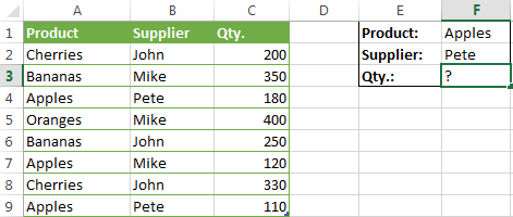
When you're learning something new, it's always a good idea to start with simple things. So, to begin with, let's define all the arguments for our SUMIFS formula:
- sum_range - C2:C9
- criteria_range1 - A2:A9
- criteria1 - "apples"
- criteria_range2 - B2:B9
- criteria2 - "Pete"
Now assemble the above parameters, and you will get the following SUMIFS formula:
=SUMIFS(C2:C9, A2:A9, "apples", B2:B9, "Pete")
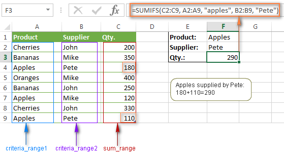
To refine the formula further, you can replace the text criteria "apples" and "Pete" with cell references. In this case, you won't have to change the formula to calculate the quantity of other fruit from a different supplier:
=SUMIFS(C2:C9, A2:A9, F1, B2:B9, F2)
Note. Both the SUMIF and SUMIFS functions are case-insensitive by nature. To get them to recognize the text case, please see Case-sensitive SUMIF and SUMIFS formula in Excel.
SUMIF vs. SUMIFS in Excel
Since the aim of this tutorial is to cover all possible ways to sum values by several conditions, we will discuss formula examples with both functions - Excel SUMIFS and SUMIF with multiple criteria. To use them correctly, you need to clearly understand what these two functions have in common and in what way they are different.
While the common part is clear (similar purpose and parameters), the differences are not so obvious, though very essential.
There are 4 major differences between SUMIF and SUMIFS:
- Number of conditions. SUMIF can evaluate just one condition at a time while SUMIFS can check for multiple criteria.
- Syntax. With SUMIF, the sum_range is the last and optional argument - if not defined, the values in the range argument are summed. With SUMIFS, sum_range is the first and required argument.
- Size of ranges. In SUMIF formulas, sum_range does not necessarily have to be of the same size and shape as range, as long as you have the top left cell right. In Excel SUMIFS, each criteria_range must contain the same number of rows and columns as the sum_range argument.
For example, SUMIF(A2:A9,F1,C2:C18) will return the correct result because the leftmost cell in the sum_range argument (C2) is right. So, Excel will make the correction automatically and include as many columns and rows in sum_range as there are in range.
A SUMIFS formula with unequally sized ranges will return a #VALUE! error.
- Availability. SUMIF is available in all Excel versions, from 365 through 2000. SUMIFS is available in Excel 2007 and higher.
Alright, enough strategy (i.e. theory), let's get into the tactics (i.e. formula examples : )
How to use SUMIFS in Excel - formula examples
A moment ago, we discussed a simple SUMIFS formula with two text criteria. In the same manner, you can use Excel SUMIFS with multiple criteria expressed by numbers, dates, logical expressions, and other Excel functions.
Example 1. Excel SUMIFS with comparison operators
In our fruit suppliers table, suppose, you want to sum all deliveries by Mike with Qty. 200 or more. To do this, you use the comparison operator "greater than or equal to" (>=) in criteria2 and get the following SUMIFS formula:
=SUMIFS(C2:C9,B2:B9,"Mike",C2:C9,">=200")
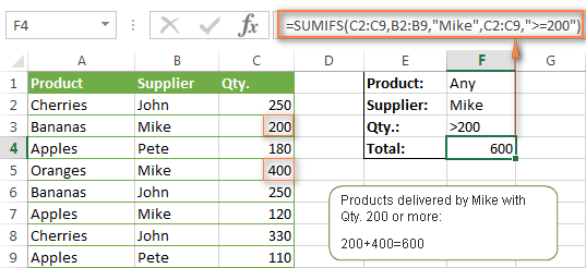
Note. Please pay attention that in Excel SUMIFS formulas, logical expressions with comparison operators should always be enclosed in double quotes ("").
We covered all possible comparison operators in detail when discussing Excel SUMIF function, the same operators can be used in SUMIFS criteria. For example, the following formula with return the sum of all values in cells C2:C9 that are greater than or equal to 200 and less than or equal to 300.
=SUMIFS(C2:C9, C2:C9,">=200", C2:C9,"<=300")
Example 2. Using Excel SUMIFS with dates
In case you want to sum values with multiple criteria based on the current date, use the TODAY() function in your SUMIFS criteria, as demonstrated below. The following formula sums values in column D if a corresponding date in column C falls within the last 7 days, including today:
=SUMIFS(D2:D10, C2:C10,">="&TODAY()-7, C2:C10,"<="&TODAY())
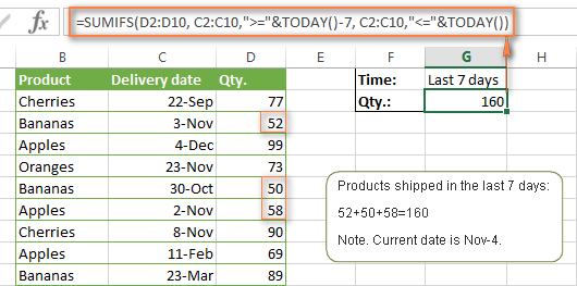
Note. When you use another Excel function together with a logical operator in the criteria, you have to use the ampersand (&) to concatenate a string, for example "<="&TODAY().
In a similar fashion, you can use the Excel SUMIF function to sum values in a given date range. For example, the following SUMIFS formula adds the values in cells C2:C9 if a date in column B falls between 1-Oct-2014 and 31-Oct-2014, inclusive.
=SUMIFS(C2:C9, B2:B9, ">=10/1/2014", B2:B9, "<=10/31/2014")
The same result can be achieved by calculating the difference of two SUMIF functions, as demonstrated in this example - How to use SUMIF to sum values in a given date range. However, Excel SUMIFS is much easier and more understandable, isn't it?
Example 3. Excel SUMIFS with blank and non-blank cells
When analyzing reports and other data, you may often need to sum values corresponding either to empty or non-empty cells.
| Criteria | Description | Formula Example | |
|---|---|---|---|
| Blank cells | "=" | Sum values corresponding to blank cells that contain absolutely nothing - no formula, no zero length string. | =SUMIFS(C2:C10, A2:A10, "=", B2:B10, "=")
Sum values in cells C2:C10 if the corresponding cells in columns A and B are absolutely empty. |
| "" | Sum values corresponding to "visually" blank cells including those that contain empty strings returned by some other Excel function (for example, cells with a formula like =""). | =SUMIFS(C2:C10, A2:A10, "", B2:B10, "")
Sum values in cells C2:C10 with the same conditions as the above formula, but includes empty strings. |
|
| Non-blank cells | "<>" | Sum values corresponding to non-empty cells, including zero length strings. | =SUMIFS(C2:C10, A2:A10, "<>", B2:B10, "<>")
Sum values in cells C2:C10 if the corresponding cells in columns A and B are not empty, including cells with empty strings. |
| SUM-SUMIF or SUM / LEN |
Sum values corresponding to non-empty cells, not including zero length strings. | =SUM(C2:C10) - SUMIFS(C2:C10, A2:A10, "", B2:B10, "")
=SUM((C2:C10) * (LEN(A2:A10)>0)*(LEN(B2:B10)>0)) Sum values in cells C2:C10 if the corresponding cells in columns A and B are not empty, cells with zero length strings are not included. |
And now, let's see how you can use a SUMIFS formula with "blank" and "non-blank" criteria on real data.
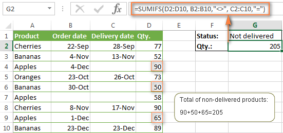
Suppose, you have an order date in column B, delivery date in column C and Qty. in column D. How do you find the total of products that have not been delivered yet? That is, you want to know the sum of values corresponding to non-empty cells in column B and empty cells in column C.
The solution is to use the SUMIFS formula with 2 criteria:
=SUMIFS(D2:D10, B2:B10,"<>", C2:C10,"=")
Using Excel SUMIF with multiple OR criteria
As noted in the beginning of this tutorial, the SUMIFS function is designed with AND logic. But what if you need to sum values with multiple OR criteria, i.e. when at least one of the conditions is met?
Example 1. SUMIF + SUMIF
The simplest solution is to sum the results returned by several SUMIF functions. For example, the following formula demonstrates how to find the total of products delivered by Mike and John:
=SUMIF(C2:C9,"Mike",D2:D9) + SUMIF(C2:C9,"John",D2:D9)
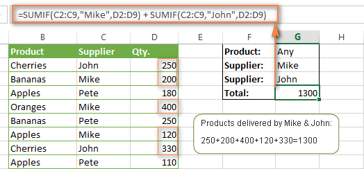
As you see, the first SUMIF function adds the quantities corresponding to "Mike", the other SUMIF function returns the amounts relating to "John" and then you add these 2 numbers.
Example 2. SUM & SUMIF with an array argument
The above solution is very simple and may get the job done quickly when there are only a couple of criteria. But a SUMIF + SUMIF formula may grow up enormously if you want to sum values with multiple OR conditions. In this case, a better approach is using an array criteria argument in the SUMIF function. Let's examine this approach now.
You can start by listing all of your conditions separated by commas and then enclose the resulting comma-separated list in {curly brackets}, which is technically called an array.
In the previous example, if you want to sum the products delivered by John, Mike and Pete, your array criteria will look like {"John","Mike","Pete"}. And the complete SUMIF function is SUMIF(C2:C9, {"John","Mike","Pete"} ,D2:D9).
The array argument consisting of 3 values forces your SUMIF formula to return three separate results, but since we write the formula in a single cell, it would return the first result only - i.e. the total of products delivered by John. To get this array-criteria approach to work, you have to use one more little trick - enclose your SUMIF formula in a SUM function, like this:
=SUM(SUMIF(C2:C9, {"John","Mike","Pete"} , D2:D9))
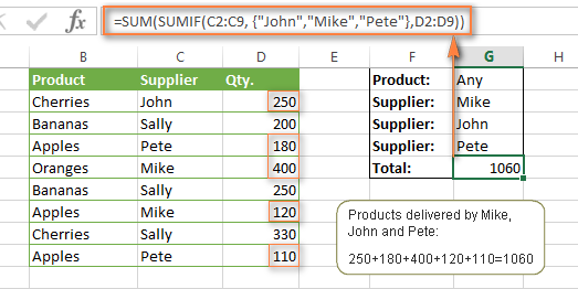
As you see, an array criteria makes the formula much more compact compared to SUMIF + SUMIF, and lets you add as many values as you like in the array.
This approach works with numbers as well as with text values. For instance, if instead of the suppliers' names in column C, you had supplier IDs like 1, 2, 3 etc., then your SUMIF formula would look similar to this:
=SUM(SUMIF(C2:C9, {1,2,3} , D2:D9))
Unlike text values, numbers needn't be enclosed in double quotes in array arguments.
Example 3. SUMPRODUCT & SUMIF
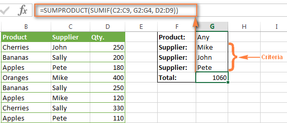
In case, your preferred way is to list the criteria in some cells rather that specify them directly in the formula, you can use SUMIF in conjunction with the SUMPRODUCT function that multiplies components in the given arrays, and returns the sum of those products.
=SUMPRODUCT(SUMIF(C2:C9, G2:G4, D2:D9))
Where G2:G4 are the cells containing your criteria, the suppliers' names in our case, as illustrated in the screenshot below.
But of course, nothing prevents you from listing the values in an array criteria of your SUMIF function if you want to:
=SUMPRODUCT(SUMIF(C2:C9, {"Mike","John","Pete"}, D2:D9))
The result returned by both formulas will be identical to what you see in the screenshot:
Excel SUMIFS with multiple OR criteria
If you want to conditionally sum values in Excel not simply with multiple OR conditions, but with several sets of conditions, you will have to use SUMIFS instead of SUMIF. The formulas will be very similar to what we've just discussed.
As usual, an example might help to illustrate the point better. In our table of fruit suppliers, let's add the Delivery Date (column E) and find the total quantity delivered by Mike, John and Pete in October.
Example 1. SUMIFS + SUMIFS
The formula produced by this approach includes a lot of repetition and looks cumbersome, but it is easy to understand and, most importantly, it works : )
=SUMIFS(D2:D9,C2:C9, "Mike", E2:E9,">=10/1/2014", E2:E9, "<=10/31/2014") +

SUMIFS(D2:D9, C2:C9, "John", E2:E9, ">=10/1/2014", E2:E9, "<=10/31/2014") +

SUMIFS(D2:D9, C2:C9, "Pete", E2:E9, ">=10/1/2014" ,E2:E9, "<=10/31/2014")
As you see, you write a separate SUMIFS function for each of the suppliers and include two conditions - equal to or greater than Oct-1 (">=10/1/2014",) and less than or equal to Oct 31 ("<=10/31/2014"), and then you sum the results.
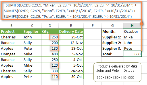
Example 2. SUM & SUMIFS with an array argument
I've tried to explain the essence of this approach in the SUMIF example, so now we can simply copy that formula, change the order of arguments (as you remember it is different in SUMIF and SUMIFS) and add additional criteria. The resulting formula is more compact than SUMIFS + SUMIFS:
=SUM(SUMIFS(D2:D9,C2:C9, {"Mike", "John", "Pete"}, E2:E9,">=10/1/2014", E2:E9, "<=10/31/2014"))
The result returned by this formula is exactly the same as you see in the screenshot above.
Example 3. SUMPRODUCT & SUMIFS
As you remember, the SUMPRODUCT approach differs from the previous two in the way that you enter each of your criteria in a separate cell rather that specify them directly in the formula. In case of several criteria sets, the SUMPRODUCT function won't suffice and you will have to employ ISNUMBER and MATCH as well.
So, assuming that the Supplies Names are in cells H1:H3, Start Date is in cell H4 and End Date in cell H5, our SUMPRODUCT formula takes the following shape:
=SUMPRODUCT(--(E2:E9>=H4), --(E2:E9<=H5), --(ISNUMBER(MATCH(C2:C9, H1:H3,0))), D2:D9)
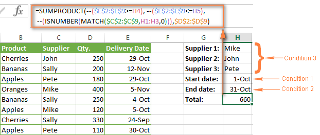
Many people wonder why use double dash (--) in SUMPRODUCT formulas. The point is that Excel SUMPRODUCT ignores all but numeric values, while the comparison operators in our formula return Boolean values (TRUE / FALSE), which are non-numeric. To convert these Boolean values to 1's and 0's, you use the double minus sign, which is technically called the double unary operator. The first unary coerces TRUE/FALSE to -1/0, respectively. The second unary negates the values, i.e. reverses the sign, turning them into +1 and 0, which the SUMPRODUCT function can understand.
I hope the above explanation makes sense. And even if it doesn't, just remember this rule of thumb - use the double unary operator (--) when you are using comparison operators in your SUMPRODUCT formulas.
Using Excel SUM in array formulas
As you remember, Microsoft implemented the SUMIFS function in Excel 2007. If someone still uses Excel 2003, 2000 or earlier, you will have to use a SUM array formula to add values with multiple AND criteria. Naturally, this approach works in modern versions of Excel 2013 - 2007 too, and can be deemed an old-fashioned counterpart of the SUMIFS function.
In the SUMIF formulas discussed above, you have already used array arguments, but an array formula is something different.
Example 1. Sum with multiple AND criteria in Excel 2003 and earlier
Let's get back to the very first example where we found out a sum of amounts relating to a given fruit and supplier:

As you already know, this task is easily accomplished using an ordinary SUMIFS formula:
=SUMIFS(C2:C9, A2:A9, "apples", B2:B9, "Pete")
And now, let's see how the same task can be fulfilled in early "SUMIFS-free" versions of Excel. First off, you write down all the conditions that should be met in the form of range="condition". In this example, we have two range/condition pairs:
Condition 1: A2:A9="apples"
Condition 2: B2:B9="Pete"
Then, you write a SUM formulas that "multiplies" all of your range/condition pairs, each enclosed in brackets. The last multiplier is the sum range, C2:C9 in our case:
=SUM((A2:A9="apples") * ( B2:B9="Pete") * ( C2:C9))
As illustrated in the screenshot below, the formula perfectly works in the latest Excel 2013 version.
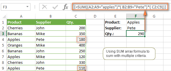
Note. When entering any array formula, you must press Ctrl + Shift + Enter. Once you do this, your formula gets enclosed in {curly braces}, which is a visual indication that an array formula is entered correctly. If you try typing the braces manually, your formula will be converted to a text string, and it won't work.
Example 2. SUM array formulas in modern Excel versions
Even in modern versions of Excel, the power of the SUM function should not be underestimated. The SUM array formula is not simply gymnastics of the mind, but has a practical value, as demonstrated in the following example.
Suppose, you have two columns, B and C, and you need to count how many times column C is greater than column B, when a value in column C is greater or equal to 10. An immediate solution that comes to mind is using the SUM array formula:
=SUM((C1:C10>=10) * (C1:C10>B1:B10))
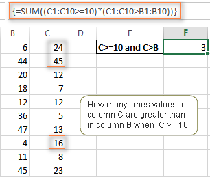
Don't see any practical application to the above formula? Think about it in another way : )
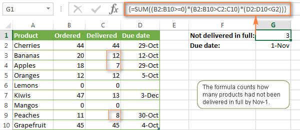
Suppose, you have the orders list like shown in the screenshot below and you want to know how many products have not been delivered in full by a given date. Translated into Excel's language, we have the following conditions:
Condition 1: A value in column B (Ordered items) is greater than 0
Condition 2: A value in column C (Delivered) in less than in column B
Condition 3: A date in column D (Due date) is less than 11/1/2014.
Putting the three range/condition pairs together, you get the following formula:
=SUM((B2:B10>=0)*(B2:B10>C2:C10)*(D2:D10<G2))
Well, the formula examples discussed in this tutorial have only scratched the surface of what Excel SUMIFS and SUMIF functions can really do. But hopefully, they have helped pointing you in the right direction and now you can sum values in your Excel workbooks no matter how many intricate conditions you have to consider.
 by
by
666 comments
Hi, I have an issue in defining a formula to sum different rows in a matrix based on different filters:
Date 29/12/2022 29/01/2023 29/01/2024 29/01/2025
Flow -189.110,0 5.890,0 5.890,0 5.890,0
Key 122022 12023 12024 12025
Date 29/12/2022 16/09/2023 16/09/2024 16/09/2025
Flow -175.723,4 6.317,5 6.317,5 196.317,5
Key 122022 92023 92024 92025
I have a matrix like this (sorry for the format): I have to define a formula to sum the "Flow" row based on the key field. Say I have to build a cash flow report, so I have all the month for a year and for each month I have to sum the different flows through the "Key" row. Is there a formula without repeating sumif for all the lines?
Many thanks for any help.
Alberto
Hi! SUMIFS function cannot sum over columns. So try the SUMPRODUCT function. I'm not quite sure how your data is organized, but the formula might look something like this:
=SUMPRODUCT((B3:N3=12022)*(MONTH(B1:N1)=1)*(YEAR(B1:N1)=2023)*B2:N2)
If this is not what you wanted, please describe the problem in more detail.
How do I ask Excel to give a sum or count for data like the below? For the below, I would want a count of 1 because all activity occurred roughly at the same time. I don't want to count each row as its own instance but rather count them as one singular event.
StationName TransactionDateTime TransactionType MedID DrawerSubDrawerPocket Quantity
G3SE 1/1/2023 9:21 Refill 64573 Drw 3.14-Pkt 2 3
G3SE 1/1/2023 9:21 Refill 64573 Drw 3.14-Pkt 1 3
G3SE 1/1/2023 9:21 Refill 64573 Drw 3.14-Pkt 3 0
G3SE 1/1/2023 9:22 Refill 64573 Drw 3.9-Pkt 2 1
G3SE 1/1/2023 9:22 Refill 64573 Drw 3.9-Pkt 4 0
G3SE 1/1/2023 9:22 Refill 64573 Drw 3.9-Pkt 1 2
G3SE 1/1/2023 9:22 Refill 64573 Drw 3.9-Pkt 3 0
Hi! Set the time interval at which all events can be counted as one. Use these guidelines: Excel SUMIFS date range formula - sum if between two dates. Pay attention to the following paragraph of this article: Sum if between two dates and another criteria.
Hi All,
From the example:
=SUM(SUMIF(C2:C9, {"John","Mike","Pete"} , D2:D9))
If i want to store the set of criteria in a cell how would i do that, when swap the criteria for a cell, and paste the values into the cell it does not work, so:
=SUM(SUMIF(C2:C9, A1, D2:D9))
In cell A1 - {"John","Mike","Pete"}
or "John","Mike","Pete"
Any ideas?
Hi! The SUMIF function cannot get an array of values from a cell. You can use a cell reference that contains only one value.
For example,
=SUM(SUMIF(C2:C9, A1, D2:D9),SUMIF(C2:C9, A2, D2:D9))
where A1 - John. A2 - Mike
You can use the TEXTSPLIT function which will return an array of text values from a cell using a separator. For example,
=SUM(SUMIF(C2:C9,TEXTSPLIT(A1," "),D2:D9))
where A1 - John Mike Pete
Been Trying this out since Wednesday, and you just solved the puzzle.
Thanks alot sir!
Alexander Trifuntov (Ablebits Team)
Hi,
I want to sum Hours!C8:C373 (this is employee time off hours)
If Hours!D8:D373 (this is the time off ID code)
= Summary!D4 (this is the time off ID I'm looking for)
And Summary!C5 (this is the employee name whose info I'm looking for)
= Hours!C7 (employee name and column header)
I tried this =IF(C5=Hours!C7,SUMIF(Hours!$D$8:$D$373,F$4,Hours!$C$8:$C$373),"") on the Summary sheet and it works.
Is there a better way? Thanks
Hi! You can use SUMPRODUCT instead of SUMIF, but you will get the same result. The formula might look something like this:
IF(C5=Hours!C7,SUMPRODUUCT((--(Hours!$D$8:$D$373=F$4))*Hours!$C$8:$C$373),"")
For more information, please read: Excel SUMPRODUCT function with multiple criteria.
IS the following formula correct:
=SUMIFS(D60:D1549,("4" ,TEXT(D60:D1549,"mm")))
please write the correct one.
Thanks so much.
Hi! The SUMIFS function cannot use other functions or expressions as arguments. Only values or cell references can be arguments to this function. I can't fix the formula as I don't know what you want to do.
HI.
I have something like this
SUM(SUMIFS(Sheet1!D:D,Sheet1!A:A,"ABC",Sheet1!K:K,{"CTA","LoB"},Sheet1!T:T,{"Delivery Complete","In Progress","Backlog"})))
My formula is not working properly.
Any solutions to this is appreciated.
Hi!
The SUMIFS function cannot use an array as a criterion. Replace {"CTA","LoB"} and {"Delivery Complete", "In Progress", "Backlog"} with OR logic, as described in the article above.
SUM(SUMIFS(Sheet1!D:D,Sheet1!A:A,"ABC",Sheet1!K:K,"CTA",Sheet1!T:T,"Delivery Complete"))) + SUM(SUMIFS(Sheet1!D:D,Sheet1!A:A,"ABC",Sheet1!K:K,"CTA",Sheet1!T:T,"In Progress"))) + ........
Hello, Please help and thank you in advance!!
=IF(D4:D7="KHR",E4:E7/4000,SUMIF(F4:F7,"Red",E4:E7))
Hi! I don't know what you want to do, but note that D4:D7="KHR" returns an array of 4 values. Your formula cannot work.
Hello, I have a data table with 3 parameters(columns for tonnage ex 1,2,..., another w two options( yes/no), and a row with categories. The matrix of the table are results of the above parameters (ex: 1,no,category-> ## or 1, yes, category-> ##(different from 1st)). I'm trying to simplify everything by having dropdown boxes for each parameter and then using sumiffs to get to the value associated with the combined parameters. I've been trying to use the sumiff function and the results do not replicate. Any help is welcomed
Sorry, it's not quite clear what you are trying to achieve. To ensure clear understanding of your task, can you provide an example of the source data and the desired result you are aiming for?
Hi, i'm trying to use the SUMIFS / SUM Array but I can't get it working, hope you can help me.
I want to have the sum of amount with the following 3 conditions;
for example: The Sum of GL account: 4000 Salaries ,Cost center: General, Period: 2023-1
1. Column G/L Account
2. Cost Center:
3. Period
This is the formula that i applied: {=SUM(A2:A12="'4000 - Gross salaries NL")*(C2:C12="'GEN MGT")*(D2:D12="2023-1")*(B2:B12)}
Hi!
I cannot check your formula as I do not have your data. However, if you have dates written in column D, then use such criteria:
(YEAR(D2:D12)=2023)*(MONTH(D2:D12)=1)
Hello. Please help as im using below formula to get the sum of 3 certain cell ranges containing "BR" and "Y" but I would also like to get the sum of the same cell ranges but containing "CH" and "N" to be added to the first formula. I've used below but the total doesn't give me the right number I'm looking for.
=SUMIFS(F25:F51,I25:I51,"BR",K25:K51,"Y")+SUMIFS(F25:F51,I25:I51,"CH",K25:K51,"N")
Hi!
Unfortunately, I don't have your data and can't check this formula. But it looks like it is correct.
How would I write a modified formula for the example using this base formula.
=SUM(SUMIF(C2:C9, {"John","Mike","Pete"} , D2:D9))
What if I wanted to another set of criteria for "products" to include "cherries" and "apples".
Essentially, I want the sum of the cross section of 2 sets of criteria in 2 separate criteria ranges. Ideally, I would like to do cell references for the criteria against its range and not hard code the criteria.
Hi!
The information you gave is not enough to give you specific advice or a formula. But I think you will find the answer to your question in this article: How to use Excel COUNTIFS and COUNTIF with multiple criteria.
Here is the brake down: want a SUMIFS formula that considers the following. I want the sum total of all the cross-sections of 3) & 5)
1) SUM RANGE: ABC'!CP:CP
2) Criteria_range1: ABC'!$C:$C
3) criterion1 (range): A7:A8
4) Criteria_range2: ABC'!$F:$F
I hope that makes sense.
5) criterion1 (range): XYZ'!$C:1$C3
Hi!
If you use your data in the instructions, which you could read yourself in the article above, we will get the formula
=SUMIFS(ABC'!CP:CP,C:C,A7,ABC'!C:C,A8,ABC'!F:F,XYZ'!C1,F:F,XYZ'!C2,F:F,XYZ'!C3)
Thanks for the reply!
However, when I input that formula (which I have tried before) the result returned is "0".
Maybe it has to do with the fact that I am using Gsheets vs. Excel?
I can't check formula because I don't have your data. I recommend reading this guide: Google Sheets SUMIFS to sum cells with multiple AND / OR criteria.
How to use SUMIF formula to collect value for same criterion from multiple sheets in same workbook.
E.g., Criterion is "TDS 22-23" in column B, Range is column A and value is in column C.
Value to be summed in from sheet 1 to sheet 4 of workbook in sheet 5.
Kindly help. Thanks
Hello!
For each sheet, use a separate SUMIF function. Here is an example formula:
=SUMIF(Data1!B2:B10, B3, Data1!C2:C10)+SUMIF(Data2!B2:B10, B3, Data2!C2:C10)
For more information, read: How to SUMIF between two sheets and SUMIF multiple columns.
Hey! I have two columns that I am working with: GL Account | Amount
The first part of the formula is fine which is =sum(sumif(B:B,{"GL Account","GL Account","GLAccount"},D:D))
The problem I am running into is that for one of the accounts I only want the number if it is equal to or > than 0 so to the above formula i tried +sumif(B:B,"GL Account",D:D,">=0") but had no luck.
Please help!
Hi!
If you have many criteria, use the SUMIFS function:
=SUMIFS(D:D,B:B,"GL Account",D:D,">=0")
For more information and examples, see article above.
I need to count minutes with 3 criteria:
I need to Sum the number of minutes (D cell) if A cell includes text with the required hotel name
and the time between 08:00 - 19:59 (and 20:00 - 07:59)
My columns:
A(Hotel name) B(Start Time) C(End Time) D(Duration)
AHotel Blabla 17:03:43 17:04:43 1
BHotel Blabla 17:02:43 17:04:43 2
AHotel Blabla 08:03:43 08:04:43 1
CHotel Blabla 08:02:43 08:04:43 2
I am trying:
=SUMIFS(D:D,A:A,"*AHotel*",B:B,">=08:00:00",B:B,"<=19:59:00")
It doesn't work, please help me...
Hello!
To set the time in the SUMIFS function, you can use TIMEVALUE function:
=SUMIFS(D2:D5,A2:A5,A2,B2:B5, ">="&TIMEVALUE("08:00:00"),C2:C5, "<="&TIMEVALUE("20:00:00"))
Hello,
I am trying to total 2 sets of values, but only if their checkboxes are checked. I have a set of checkboxes in cells B9, B11, B13 & B15 and values for these in column E, and another set of checkboxes in cells B26, B28 & B30 with their values also in column E.
For the first set I have written the formula =SUMIFS(E8:E15, B8:B15, TRUE) in cell F16, which works. However, I only want this to calculate if none of the checkboxes in cells B26, B28 & B30 are checked. What formula should i use instead?
Also, the values for the second set only need to be included in the total too, if all B9, B11, B13 & B15 checkboxes in the first set are checked, so for this I have written the formula =IF(AND(B9=TRUE,B11=TRUE,B13=TRUE,B15=TRUE),SUM(E8:E15),"") in cell F31, which also works.
However I want to also include the values of the second set in cell F31 too, but only if their checkboxes (B26, B28 & B30) are also checked. What formula should I use for this?
Hello!
Use the IF AND statement to calculate SUMIF if three conditions are met.
Try this formula
=IF(AND(B26=FALSE,B28=FALSE,B30=FALSE),SUMIFS(E8:E15,B8:B15,TRUE),"")
Hi Alexander,
Brilliant as ever, that works great, thanks!
Scenario:
Given data are availment dates, transactions and amounts per transaction
I wanted to summarize the total for each dates and I have managed to use the =SUMIFS formula.
However, I wanted to drag down the formula for the rest of the transaction dates and failed have the correct total.
What should I do with my formula?
TIA
Hi!
The following tutorial should help: How to copy formula in Excel with or without changing references.
How can I make this formula below work without having to type/copy/Paste "180/470/560100704-Grants from State Agen" in the formula. I tried to do it with a reference to the cell Directly to the Left "B4" with the exact text of "180/470/560100704-Grants from State Agen" but the formula didn't work. I built this formula but i am sort of a novice at this. There are hundreds of lines that have different codes and text so it is better if i can reference the cell "B4" to make the formula work. A different formula is OK but this is how i figured out how to do this.
Essentially i have 3,000 lines of a general ledger that i want to summarize into there perspective monthly entries.
L2 = 2022
L3 = October
=SUMIFS(DATA!$G$3:$G$6000,DATA!$C$3:$C$6000,"180/470/560100704-Grants from State Agen",DATA!$E$3:$E$6000,SUMMARY!L3,DATA!$A$3:$A$6000,SUMMARY!L2)
Hi!
I can't check your formula because I don't have your data. If the text in the cell is written correctly, the formula will work. Check carefully what is written in the cell. For more information, please visit: How to correctly use cell references in SUMIF criteria.
Thank you that detail (">"B4,)worked. But. It is Suming the entire column it is referencing without considering the other "Ifs" Aka Year(L2) and Month(L3).
To sum not the whole column, add conditions to the SUMIFS formula. You can find all the information you need in the article above. To compare not the whole date, but only the month or year, use the MONTH or YEAR functions.
Let me elaborate more. The Formula is Looking at Tab "DATA" at Column C ("C3:C6000") for the Info on B4 (B4 is matching C3:C6000) and Returning info form Column G. It is also checking for a match in L2 and L3 for info in the Data TAB for Column E and A.
=SUMIFS(DATA!$G$3:$G$6000,
DATA!$C$3:$C$6000,
"180/470/560100704-Grants from State Agen",
DATA!$E$3:$E$6000,
L3,
DATA!$A$3:$A$6000,
L2)
I want to Replace "180/470/560100704-Grants from State Agen" with a Reference to B4 which you showed me ">"B4. But when i do this instead of returning a summary of $2,734 it is giving me 73,456. This i assume is a summary of the entire column of G Rather than just column G in October of 2022.
=SUMIFS(DATA!$G$3:$G$6000,
DATA!$C$3:$C$6000,
">"$B4,
DATA!$E$3:$E$6000,
L3,
DATA!$A$3:$A$6000,
L2)
Hello.
What I am looking for is means to SUM values based on their concomitant criteria not being part of values already summed up elsewhere...
e.g.
[A] [B]
[1] Bob 100
[2] Bob 200
[3] Sue 350
[4] Tom 220
[5] Bill -130
[6] Jane -240
[7] Jane -87
COUNTA for COL[A] is going to be 7
SUM for COL[B] is going to 413
The grand total needs to be calculated, but values under 0 need to be excluded elsewhere for writing out concatenated text values.
It took forever to do this using SUM, COUNTA, COUNTIF functions and a separate equation as a name range. But that was so clunky... 😒😯
My main problem is dealing with SUM for multiple COUNTIF statements.
Thank you.
Hello!
I don't quite understand what you want to do. However, if a cell contains text and a number, you cannot do math. Extract the number into a separate cell. Here are the instructions: Extract number from text string.
Thank you for detailed blog. I am looking for a formula to calculate total qty product wise in column E and F. for example.
Apples 410
Bananans 600
Cherries 530
Oranges 400
Can you please help?
Hi!
Have you tried the ways described in this blog post? If they don’t work for you, then please describe your task in detail.
What if I need a 2nd column data pulled? I currently have this formula but need to add an additional data info from a range of columns (from Sanchez!B8:B7)
=SUMIFS(Sanchez!C8:C67,Sanchez!A8:A67,"<="&Summary!M7)
Hi!
If I understand your task correctly, try the following formula:
=SUMIFS(Sanchez!C8:C67,Sanchez!A8:A67,"<="&Summary!M7)+SUMIFS(Sanchez!B8:B67,Sanchez!A8:A67,"<="&Summary!M7)
Please read the above article carefully.
In the Example Example 3. SUMPRODUCT & SUMIFS with Mike, John and Pete in column H,
how can you use a single sumproduct function or other function in cell I1 to get the total broken down by Mike, John and Pete?
SUMIFS can do this, but SUMIFS does not allow other functions within the ranges or criteria.
It would look like this, the cell with 120 has the single formula that spills down based upon the number of items in column H.
H I
Mike 120
John 250
Pete 290
i need formula to sum a column in a table based on which are details in two coloumns were nill and i need to make sure there is another column must include a specific text.please help
I am not sure I fully understand what you mean.
Hi,
If there's any text in QTY cell, how i will SUMIF by criteria? i mean i need to ignore text's in QTY column and sum the values in QTY column with a criteria i have in another sheet.
Thanks
Hi!
Text values are ignored by the SUMIF function.
Hi, is it somehow possible to use different size range lengths in SUMIFS
for example, i have values in the range a1:a10 and i want to sum these values based on two different criteria.
criteria 1 range=b1
criteria 1 = "city"
criteria 2 range=c1
criteria 2 = "yes"
=sumifs(a1:a10,b1,"city",c1,"YES")
this is only a dummy example, i have multiple sheets in which i have to use this kind of values.
this can be done using the helper column(in every sheet i have to create a helper column), but i want it without a helper column. (maybe possible...)
thanks
Hi!
Is not possible to use different size range lengths in SUMIFS.
thanks for replay
any workaround for this problem,,, maybe any other formula for this??
How do I use TRIM formula within SUMIFS formula to clear invisible spaces??
Hi!
You cannot use any function inside the SUMIFS function. To calculate a conditional sum, use the SUMPRODUCT function. Please have a look at this article Excel SUMPRODUCT function with formula examples.
Great place to learn excel
I have a query
let's say I have a list of 1000 ordered however, my previous inventory is divided into sets of 100 and each set of 100 units has a unique landing cost now I want to know how I can enter these costs in a formula
example
Column A is the list of 1000 order and each cell in the column is having either 1 or 2 written
Column B needs to add landing cost which is unique for each set of 100 units so It means I have 10 different landing cost
Please share a formula that can automate the process
Hi!
To find the cost by unit name, you can use the VLOOKUP or INDEX MATCH formula.
The information you provided is not enough to understand your case and give you any specific advice, sorry.
sum should equal 20. You should use the + operator
Hello Sir,
Is there any shortcut for this formula
SUMIFS(Net_Delivery21,CODE21,A6)+SUMIFS(Net_Delivery21,CODE21,B6)+SUMIFS(Net_Delivery21,CODE21,C6)+SUMIFS(Net_Delivery21,CODE21,D6)+SUMIFS(Net_Delivery21,CODE21,E6)
Thanks
sorry I mean this one Sir,
SUMIFS(Z2:Z500,A2:A500,A6)+SUMIFS(Z2:Z500,A2:A500,B6)+SUMIFS(Z2:Z500,A2:A500,C6)+SUMIFS(Z2:Z500,A2:A500,D6)+SUMIFS(Z2:Z500,A2:A500,E6)
Thanks
Hi!
If you are interested in shortcuts, I recommend this article: 30 most useful Excel shortcuts.
Hi!
As your instruction, we have
1. =SUMPRODUCT(SUMIF(C2:C9, {"Mike","John","Pete"}, D2:D9))
2. =SUMPRODUCT(SUMIF(C2:C9, G2:G4, D2:D9))
I try to find how I can replace "Pete" in formula 1 into G4 (as the value of G4 is Pete) , the formula would become
=SUMPRODUCT(SUMIF(C2:C9, {"Mike","John",G4}, D2:D9))
but it doesn't work, pls help me how fix it!! B/c I want to create an array from specific text and from value of cell
Tks!!!
Hello!
You cannot use cell references in an array of values.
Use the SUMPRODUCT function with multiple conditions.
=SUMPRODUCT(D2:D9,(C2:C9=G3)+(C2:C9=G4))
How to SUM the Qty automatically in MS Office 2007 Excel if OD, THK & SPECN changed.
DESCN OD THK SPECN Qty
Pipe 60.30 5.54 SA 106 GR B 28.26
Pipe 60.30 5.54 SA 106 GR B 24.6
Pipe 88.90 5.49 SA 106 GR B 3
Pipe 88.90 5.49 SA 106 GR B 46.632
Pipe 88.90 7.62 SA 106 GR B 11.52
Pipe 88.90 7.62 SA 106 GR B 2
Pipe 88.90 7.62 SA 106 GR B 3
Pipe 88.90 7.62 SA 106 GR B 3
Pipe 88.90 7.62 SA 106 GR B 46.048
Pipe 88.90 7.62 SA 106 GR B 38.6
Pipe 88.90 11.13 SA 106 GR B 6.2
Pipe 114.30 6.02 SA 106 GR B 1
Pipe 114.30 8.56 SA 106 GR B 7.26
Pipe 114.30 8.56 SA 106 GR B 3
Pipe 114.30 8.56 SA 106 GR B 3
Pipe 114.30 8.56 SA 106 GR B 182.848
Pipe 114.30 8.56 SA 106 GR B 0.7
Pipe 114.30 8.56 SA 106 GR B 0.7
Hi!
Have you tried the ways described in this blog post? If they don’t work for you, then please describe your task in detail, I’ll try to suggest a solution.
Great work, explain everything very clear with simple example. Thanks alot.
Thanks very much for this great tutorial! I'm trying to create a formula that is a bit beyond my basic skill set and hoping you could provide guidance. I'm trying to pull data from one sheet into another, with multiple parameters as follows:
One one sheet ("Data 2") I have "$ revenue" in column O and "Campaign Name" in column P " -
So it looks a bit like this:
Column O. Column P
$100. Campaign A
$50. Campaign A
$75. Campaign A
$250. Campaign B
etc.
I'm trying to put that into a summary sheet, to sum up revenue by campaign - and match by Campaign Name on that summary sheet (column B).
So it looks like this
Col B: Campaign Name Revenue
Campaign A. (formula here should = $225)
Campaign B. etc.
I came up with this: =SUMIF('Data 2'!O:O,B:B,'Data 2'!P:P)
(hit send too soon!) - but that formula is giving me a $0 result for some reason.
Also, to make things more complex, I'd like to also suppress certain sales stages (sheet Data 2, column Q) from being included. I've tried this, but also is not working (error message, so definitely wrong..):
=SUMIF('Data 2'!O:O,B:B,'Data 2'!P:P,'Data 2'!Q:Q"Closed Nurture","Closed Won","Closed Lost")
Hi!
Please re-check the article above since it covers your task.
If I understand correctly, the formula might look like this:
=SUMIFS(‘Data '2′'!O:O,’Data '2′'!P:P,B1,’Data '2’'!Q:Q,”<>Closed Nurture”,’Data '2’'!Q:Q,”<>Closed Won”,’Data '2’'!Q:Q,”<>Closed Lost”)
Thank you! That looks exactly right - but I'm still getting a "formula parse error" (?)
Hi!
I can't check the formula that contains unique references to your workbook worksheets. I have shown you how to modify your formula. Use SUMIFS function.
Hello!
SUMIF function cannot return an array of values. SUMIF can only sum by one criterion.
=SUMIF(‘Data 2′!O:O,B1,’Data 2’!P:P)
You can copy this formula down along the column.
You can create a pivot table using this instruction: How to make and use PivotTables in Excel.
HI I HAVE FORMULA AS BELOW,
HOW TO sum up column I only when the value of Column I is less than zero?
=SUMIFS('DD Policy Due'!I:I,'DD Policy Due'!H:H,Consolidated!D3) * IF(G3="D",1,-1)
Hi!
To find the sum of the values in a column that is less than 0, use these guidelines: How to use SUMIF function in Excel with formula examples.
For example,
=SUMIF(I:I," < 0",I:I)
Thank you so much but how could I incorporate with my Formula?
=SUMIFS('DD Policy Due'!I:I,'DD Policy Due'!H:H,Consolidated!D3) * IF(G3="D",1,-1)
When I am typing as below error is coming
=SUMIFS('DD Policy Due'!I:I,"<0",'DD Policy Due'!I:I,'DD Policy Due'!H:H,Consolidated!D3) * IF(G3="D",1,-1)
Hi!
I’m not sure I got you right since the description you provided is not entirely clear. However, it seems to me that the formula below will work for you:
=SUMIFS(I:I,I:I," < 0",H:H,D3) * IF(G3="D",1,-1)
Thank you very much for this very useful post on Excel formulas for multiple criteria requirement.
Please give me some solution for below requested formula if it is right
=SUMIFS(A2:E2,">="120000-10%)
Hi!
You don't have all function arguments filled in. Read the guide and examples above carefully.
If you only have one condition, use the SUMIF function.
Hi Alexander,
I am trying to figure out how to calculate Monthly recurring revenues when new customers coming in and others leave.
Assume all customers remain only 4 months
Month 1 2 3 4 5 6
New monthly revenues 100 300 500 700 900 1100
Monthly recurring revenues 100 400 900 1,600 2,500 ?????
How do I make sure that in month 6 I do the following?
Sum all New monthly revenues from months 1 through 6 EXCEPT months 1 and 2 because the time that has passed by is greater than 4 months?
Thank you
-
Hello!
If you need to use a formula in the summation condition, then use the SUMPRODUCT function to calculate the sum by multiple criteria:
=SUMPRODUCT(--(A1:L1>(MONTH(TODAY())-4)),--(A1:L1<=(MONTH(TODAY()))),A2:L2)
I hope it’ll be helpful. If something is still unclear, please feel free to ask.
Dear Alexander,
1. You are my hero
2. I am forever grateful
3. Your help will make me look good in front of my colleagues!
Thank you!
Carlos
Hello, Sir kindly guide me what's the best platform for advanced excel learning and free of cost.
I used below formula and total amount = 70. Seems it only adding "Terry". I want to see the total amount of Terry, John and Pete. Am I missing something? Thanks.
=SUM(SUMIFS(B2:B10,A2:A10,{"Terry", "John", "Pete"}))
name amount
Terry $10
John $20
Terry $30
Pete $10
John $30
Lian $20
George $10
Pete $20
Terry $30
Hi!
Unfortunately, I could not get the result 70. Your formula gives a result - 150. Try to enter your formula as an array formula. Enter via Ctrl + Shift + Enter, not just Enter.
Hi
May i request anyone, how can i use cell reference in sum if instead of typing manually.
Example-: SUMIF('Jan22-29.3.22'!$AL:$AL,"*WTFL*",'Jan22-29.3.22'!$AQ:$AQ)
Question: Why need to edit the formula to type WTFL or any other word in order to get total.
Thanks
Anoop
Hello!
Replace the value in the formula with a reference to the cell that contains that value.
SUMIF(‘Jan22-29.3.22′!$AL:$AL,$A$1,’Jan22-29.3.22’!$AQ:$AQ)
A1 -- *WTFL*
i was using sumifs formula with multiple criterias. but i am unable to fetch the previous criteria data if some criteria are blank. need your support
Trying calculate the total revenue (in cells T3:T11000) IF the service type = Social (in cells D3:D11000) AND the project status = Active (in cells K3:K11000) AND the invoice date falls in between 01/01/2021 and 01/31/2021. Report totals to appear on a separate tab from the summary data on tab entitled "All Projects".
My (erroneous) attempt:
=SUMIFS('All Projects '!T3:T11000,'All Projects '!D3:D11000,"=*SOCIAL*",'All Projects '!C3:C11000,">=01/01/2021",'All Projects '!C3:C11000,"<=01/31/2021")+SUMIFS('All Projects '!T3:T11000,'All Projects '!K3:K11000,"*active*")
Can you please help? Thank You!
Hi!
Please re-check the article above since it covers your case.
Here is a sample formula for you
=SUMIFS(T3:T7,C3:C7,">01/01/2021",C3:C7,"<31/01/2021",D3:D7,"*Social*",K3:K7,"*Active*")
Dear Sir, i want to apply this condition can you help me regarding this
Excess [if (C7 = 1+1+1,3*D7*G7),(if (C7 = 1+1,2*D7*G7),if (C7 = 1,1*D7*G7),0
Dear i want to apply this condition can you help me regarding this
Excess Un-adjusted Credit [if F24 = Yes and F25 > F17 then (F25 - F17); otherwise zero; if F24 = No then (F8 - F25)]
her "F" is column and numbers are rows
Hello!
Please check out the following article on our blog, it’ll be sure to help you with your task: Excel Nested IF statement: examples, best practices and alternatives.
=IF(AND(F24="Yes",F25>F17),F25-F17,IF(F24="No",F8-F25,0))
Hi, I want to type Not Available or text when the result of Sumif or Sumifs = 0 (Zero) Please advise
Hello!
Use IF function to get the result by condition. For example:
=IF(SUMIFS(C2:C9, A2:A9, "apples", B2:B9, "Pete")=0,"Not Available",SUMIFS(C2:C9, A2:A9, "apples", B2:B9, "Pete"))
Long time follower....first time poster ;)
Trying to set something up where I can get my MTD target based on day of month input.
Example: If in Cell A1 I input '7' for the 7th day of Jan.
In say cell B9, I want it to reflect the sum of daily targets in a table on a separate sheet.
For simplicity sake: the table is C7:AG7, I would want B9 to be the SUM of C7 to I7.
I can't figure this one out
Hi!
If I understand your task correctly, the following formula should work for you:
=SUM(INDIRECT("C"&A1&":I"&A1))
You can learn more about INDIRECT function in Excel in this article on our blog.
Hi. Please I’m trying to use this formula buts it’s only recognizing the security. It’s not summing up the security and electricity.
=SUMIFS('259222496_1_59_0'!D12:D,'259222496_1_59_0'!I12:I,{"O.N- SECURITY","O.N- ELECTRICITY"},'259222496_1_59_0'!A12:A,">="&DATE(YEAR(B5),MONTH(B5),1),'259222496_1_59_0'!A12:A,"<="&EOMONTH(B5,0))
Hello!
It is very difficult to understand a formula that contains unique references to your workbook worksheets. Explain what data you are using and what result you want to get.
Also, notice the paragraph above: Using Excel SUMIF with multiple OR criteria.
{“O.N- SECURITY”,”O.N- ELECTRICITY”} - this does not work.
I want to sum up the figures with “O.N Security” and “O.N Electricity”. I haven’t able to do them individually with the formula but I’m trying to sum them together
Hi!
Read the paragraph I recommended. There is an answer to your question. I cannot write you a formula, as it contains unique references to your data, which I do not have.
Quote value Days_to_close Salesman Quote_month
234 90 Ram 01-Jan-15
342 100 Satish 05-Feb-15
122 34 Suresh 15-Apr-15
544 67 Suresh 15-Nov-15
232 99 Ramu 14-Nov-15
533 89 Babu 29-Dec-15
21 63 Suresh 01-Dec-15
SUM of Quote_Value if Salesman name is Suresh and Days_To_Close is equal to or less than 90 and Quote_Month is equal to one of the following (Oct-15, Nov-15, or Dec-15).(using formulae)
Hi!
Have you tried the ways described in this blog post? Please re-check the article above since it covers your case.
Hi,
I have jam and other stuff everywhere.
I want to know how much jam is in the larder.
So, trying to use SUMIFS, I have the following spreadsheet.
My Σrange is all the numbers; My first criterion range is all the stuff; My first criterion is stuff: My second criterion range is all the places; My second criterion is places.
It doesn’t work. Whyyyyyyy?
In reality, I’ve a Census database of 'How many speak each of 200 languages in each of UK’s 1000 regions'.
Finding how many speak something somewhere manually is a pain in the archive.
(To simplify entering the two criteria, I’ve used ‘data validation’, with an input-list for each criterion.)
Here's the spreadsheet - or it would be if it could be copied and pasted properly!
criterion 2 Larder
criterion 1 jam #VALUE! ←←
places → Larder Cupboard Fridge
stuff ↓ biscuits 10 20 3 ← numbers
butter 3 0 1
cheese 4 0 2
jam 15 5 0
……....................................................................................
Formula (in F16): SUMIFS (F19:H22, E19:E22, E14,F18:H18, F13)
[the spaces are for easier reading only]
--- In 'English': Sums if ( Σrange, C1range, C1, C2range, C2)
Hello!
All ranges of values in the SUMIFS function must be the same size. You can read about this in the article above. An example of your formula:
=SUMIFS(E19:G22, I19:K22, E14, M19:O22, F13)
I want a conditional formula for insurance calculation based on below criteria
Gender Name Age Married/Single Insurance Calculation
Male XYZ 16 Single
Male XYZ 23 Single
Male XYZ 58 Married
Female XYZ 60 Married
Female XYZ 25 Single
Male XYZ 29 Married
Female XYZ 32 Married
Criteria:
Gender/Status Amount Age
Male/single 265.00 From 5 to 19 years
Male/single 270.00 From 20 to 40 Years
Male/single 300.00 from 41 to ETC
Female/Single 270.00 From 5 to 19 years
Female/Single 300.00 From 20 to 40 Years
Female/Single 350.00 from 41 to ETC
Male/Married 300.00 From 5 to 19 years
Male/Married 350.00 From 20 to 40 Years
Male/Married 400.00 from 41 to ETC
Female/Married 337.00 From 5 to 19 years
Female/Married 388.00 From 20 to 40 Years
Female/Married 442.00 from 41 to ETC
Female/Maternity 450.00
Child 200.00
Hello!
I don't quite understand what you want to count. But in order to use the criteria in the formula, each of them must be written in a separate cell. To split a cell with criteria, use these guidelines: How to split cells in Excel.
Thanks a lot,
it's worked..