This tutorial will teach you a few easy ways to sum multiple columns in Excel based on a single or multiple criteria.
Doing a conditional sum in Excel is a piece of cake as long as all the values to be totaled are in one column. Summing multiple columns is a problem because both the SUMIF and SUMIFS functions require the sum range and criteria ranges to be equally sized. Luckily, when there is no straight way to do something, there is always a work-around :)
Excel Sum If: multiple columns, single criterion
First off, let's get to know exactly what problem we are trying to solve. Suppose you have a table of monthly sales like shown below. Because it was consolidated from a number of regional reports, there are a few records for the same product:
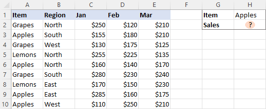
The question is - how do you get a total of sales for a certain item?
The first idea that comes to mind is using a SUMIF formula in its pure form:
=SUMIF(A2:A10, "apples", C2:E10)
Unfortunately, this won't work. The reason is that the dimensions of sum_range are determined by Excel automatically based on the dimensions of the range argument. As our criteria range includes only one column (A2:A10), so does the sum range (C2:C10). The sum_range parameter defined in the formula (C2:E10) actually determines only the upper left cell of the range that will be summed. As a result, the above formula will add up the apples sales only in column C. Not what we are looking for, eh?
The simplest working solution that suggests itself is to create a helper column summing the numbers for each individual row, and then use that column for sum_range.
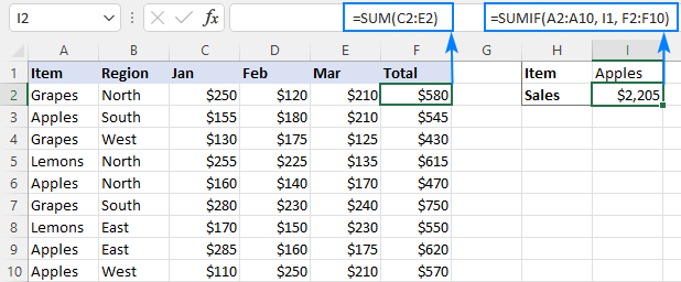
So, go ahead and place a SUM formula in F2, then drag it down across as many cells as needed:
=SUM(C2:E2)
After that, you can quickly have the job done:
=SUMIF(A2:A10, I1, F2:F10)
Where I1 is the item of interest.
In the above formula, sum_range is of the same size as range (1 column and 9 rows), so it works without a hitch:
If the layout of your worksheet does not have room for any extra columns, then apply one of the following solutions.
SUMIF multiple columns
The idea is to write a separate SUMIF formula for each of the columns you want to sum, and then add up the results:
Or
A practical implementation looks as follows:
=SUM(SUMIF(A2:A10,H1,C2:C10), SUMIF(A2:A10,H1,D2:D10), SUMIF(A2:A10,H1,E2:E10))
Or
=SUMIF(A2:A10, H1, C2:C10) + SUMIF(A2:A10, H1, D2:D10) + SUMIF(A2:A10, H1, E2:E10)
You can also "hardcode" the condition in the formula if needed:
=SUMIF(A2:A10, "Apples", C2:C10) + SUMIF(A2:A10, "Apples", D2:D10) + SUMIF(A2:A10, "Apples", E2:E10)

This works fine for a reasonable number of columns, but for a large dataset the formula becomes too long and difficult to read. In this case, the below solutions are more appropriate.
SUM as array formula
Another way to do a sum if in multiple columns based on one criterion is to construct an array formula:
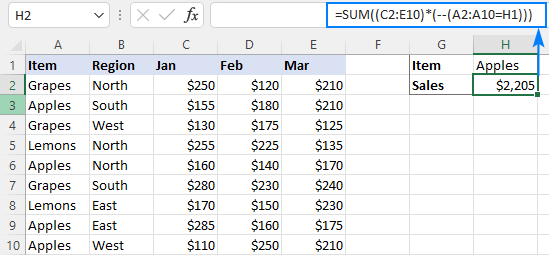
For our sample dataset, the formula takes this form:
=SUM((C2:E10)*(--(A2:A10=H1)))
Or
=SUM((C2:E10)*(--(A2:A10="Apples")))
In Excel 2019 and older, you should press Ctrl + Shift + Enter to complete the formula correctly. In Excel 365 and Excel 2021, this works as a normal formula due to inbuilt support for dynamic arrays.
How this formula works:
The core concept is to multiply the elements of these two arrays:
- (C2:E10) - all the values in the sum range. In our case, the array contains 27 elements (3 columns and 9 rows: {250,120,210;155,180,210;130,175,125; …}
- (--(A2:A10=H1)) - compares each value in A2:A10 against the target item in H1. The result is an array of TRUE (the condition is met) and FALSE (the condition is not met) values, which is then converted into an array of 1's and 0's with the help of a double unary operator: {0;1;0;0;1;0;0;1;1}
Please pay attention that the first array is two-dimensional (each column of data is separated by a comma and each row by a semicolon) and the second one is a one-dimensional vertical array (1 column of data, rows are separated by semicolons). When the two arrays are multiplied, all the items of the 2D array in a given row are multiplied by the corresponding element of the 1D array:

As multiplying by zero gives zero, only the numbers for which the criterion is TRUE survive, and the SUM function adds them up:
=SUM({0,0,0;155,180,210;0,0,0;0,0,0;160,140,170;0,0,0;0,0,0;…})
To make the formula's logic easier to understand, you can write the first multiplier in this way:
=SUM((C2:C10 + D2:D10 + E2:E10) * (--(A2:A10=H1)))
This will produce an array of sums by row (like the helper column does in the very first example), which is then multiplied by an array of 1's and 0's:
{580;545;430;615;470;750;550;620;570}*{0;1;0;0;1;0;0;1;1}
The result of multiplication is served to SUM:
=SUM({0;545;0;0;470;0;0;620;570})
Don't like using arrays formulas in your sheet? Neither do I. Well, let's go check the next solution :)
SUMPRODUCT formula
The strategy described in the above example can also be implemented using the SUMPRODUCT function.
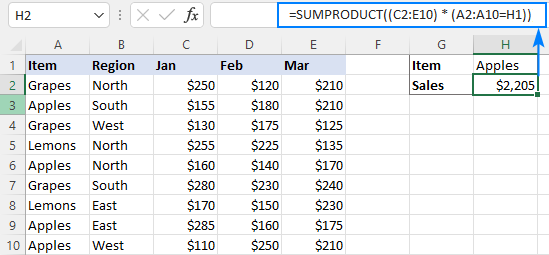
A real-life formula goes as follows:
=SUMPRODUCT((C2:E10) * (A2:A10=H1))
The formula's logic is the same as in the previous example. The beauty of the SUMPRODUCT function is that it supports arrays natively, so it works nicely as a regular formula in all Excel versions.
Excel Sum If: multiple columns, multiple criteria
The three approaches we utilized to add up multiple columns with one criterion will also work for conditional sum with multiple criteria. The formulas will just become a little more complex.
SUMIFS + SUMIFS to sum multiple columns
To sum cells that match multiple criteria, you normally use the SUMIFS function. The problem is that, just like its single-criterion counterpart, SUMIFS doesn't support a multi-column sum range. To overcome this, we write a few SUMIFS, one per each column in the sum range:
Or
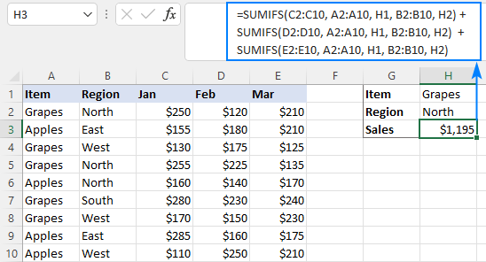
For example, to sum Grapes sales (H1) in the North region (H2), the formula is:
=SUMIFS(C2:C10, A2:A10, H1, B2:B10, H2) + SUMIFS(D2:D10, A2:A10, H1, B2:B10, H2) + SUMIFS(E2:E10, A2:A10, H1, B2:B10, H2)
Array formula to conditionally sum multiple columns
The SUM formula for multiple criteria is very much like that for a single criterion - you just include additional criteria_range=criteria pair(s):
For instance, to sum sales for the item in H1 and the region in H2, the formula goes as follows:
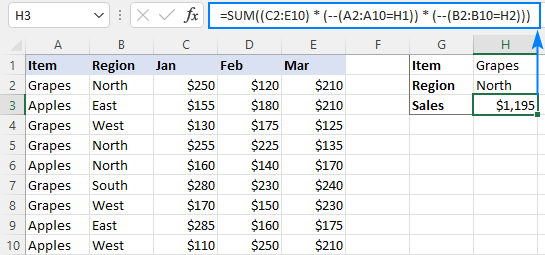
=SUM((C2:E10) * (--(A2:A10=H1)) * (--(B2:B10=H2)))
In Excel 2019 and older, remember to press Ctrl + Shift + Enter to make it an CSE array formula. In dynamic array Excel 365 and 2021, a normal formula will work fine as shown in the screenshot:
SUMPRODUCT formula with multiple criteria
The easiest way to sum multiple columns based on multiple criteria is the SUMPRODUCT formula:
As you can see, it's very similar to the SUM formula, but does not require any extra manipulations with arrays.
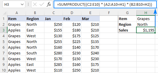
To sum multiple columns with two criteria, the formula is:
=SUMPRODUCT((C2:E10) * (A2:A10=H1) * (B2:B10=H2))
These are the 3 ways to sum multiple columns based on one or more conditions in Excel. I thank you for reading and hope to see you on our blog next week!
Practice workbook for download
Sum if multiple columns - examples (.xlsx file)
 by
by
57 comments
Just sent a query earlier and seems this one may be working:
=IF($O75="R",SUMIFS($R$3:$R$25, $AC$3:$AC$25,"*R*",$AA$3:$AA$25, N75),0) letting me use range *R*
Lovely!!!!
Excellent Website! Encountered some difficulty integrating SUMPRODUCT with different criteria when I use search *symbol*, as SUMPRODUCT seems can not see the text from range and only wants reference to the exact cell. Maybe I am moving to the wrong direction? I have only one column for if sum and two separate columns for criteria but the criteria is not the exact reference to the cell but the part of text (I am using codes, so if at least one code is picked up this is true, but as all the code are in one cell I can not use the whole range as a reference.
Original
=IF($O74="R",SUMIF($AC$3:$AC$25,"*R*",$R$3:$R$25),0)
Want to add additional search and range within SUMIF as SUMIF is ok with "*code*"
Thank you !
Hi! If you want to calculate the sum of partial text matches using SUMPRODUCT function, here is an example formula:
=SUMPRODUCT(ISNUMBER(SEARCH("R",A1:A10))*B1:B10)
You can also find useful information in this article: Excel FIND and SEARCH functions with formula examples. If this is not what you wanted, please describe the problem in more detail.
column A customer name
Column B, row 1 onwards month eg: Jan, Feb....etc
Column B row 2 onwards different product eg: Apple, grapes.
what is the suggest formula can use to sum total quantity for each coustomer in column A from Jan (to mar (based quarterly order) to forecast the trend?
Hi! There is no quantity you want to summarize in your data description. However, I’ll try to guess and offer you the following formula:
=SUMPRODUCT((A3:A11="A") * ((B3:F11) * (B2:F2="Apple") * ((B1:F1="Jan") + (B1:F1="Feb") + (B1:F1="Mar"))))
I recommend reading this guide: Excel SUMPRODUCT function with formula examples.
Hi Alexander
Thanks for suggestion.
I would like to sum total quantity of each month for each type product of each customer. As there will be has 12 months in row and 20 products for multiple customer. So would like to know sum order for each type product in each month of every customer.
Hi! In your first question, you wanted to summarize January through March. Leave only one month in the formula if you only want the amount for one month. If this formula does not work for you, please explain in detail why.
=SUMPRODUCT((A3:A11="A")*((B3:F11)*(B2:F2="Apple")*(B1:F1="Jan")))
In your example 'Array formula to conditionally sum multiple columns':
=SUM((C2:E10) * (--(A2:A10=H1)) * (--(B2:B10=H2)))
If your column A had many types of fruit and you wanted to return the total sales value of say {"Apples","Grapes","Pears"} over the 3 months irrespective of Region, how would you include this, preferably in the syntax you have used in this example?
I would also like to replace the Month names for dates e.g. 01/03/2024 which I can then format as MMM-YY, so that I can then also add a filter (--(C1:N1<=Q1), where Q1 is the month I select from a drop down list - so that I can pick up 12 months worth of year-to-date values of whichever combinations of product in column A that I want, for whichever month I want.
Can I achieve both filters in the one formula using the SUM array syntax?
Hello! To use multiple criteria in column A, the formula might look something like this:
=SUMPRODUCT((C2:E10) * ((A2:A10=H1)+(A2:A10=I1)+(A2:A10=J1)) * (--(B2:B10=H2)))
Look for the example formulas here: Excel SUMPRODUCT function with formula examples.
Also note that formatting the date as MMM-YY does not change the date value in the cell. Try to use the recommendations described in this article: Excel IF between two dates.
I hope it’ll be helpful. If something is still unclear, please feel free to ask.
had similar issue where my data was spread across multiple columns, but I only wanted to sum based on BOTH row & column criteria. The row criteria was a "single" row, so I was able to use INDIRECT combined w/MATCH to determine which row to add, then basic SUMIFS for my column criteria.
My data has item # down 1st column and weekly buckets across the top. I need to add all values w/in a month for a 'selected' item.
SUMIFS(INDIRECT("Export!"&MATCH($A2,Export!$A:$A,0)&":"&MATCH($A2,Export!$A:$A,0)),Export!$1:$1,">="&'Open and Planned'!C$1,Export!$1:$1,", =, <.
Does anyone have another/easier way to achieve the same?
looks like part of my message cut off. my formula is SUMIFS(INDIRECT("export!"&MATCH($A2,Export!$A:$A,0)&":"&MATCH($A2,Export!$A:$A,0)),Export!$1:$1,">="&'Open and Planned'!C$1,Export!$1:$1,"<"&'Open and Planned'!D$1)
where Export is the worksheet name that contains the sum range, cell A2 is the item #, cells C1/D1 are the start/end dates to check
Hi Alexander, how can I replace the '=' in criteria with to indicate a range - my formula returns #VALUE!
Sample of my formula shown below
=SUM((D:O)*(--(B:B>1099))*(--(B:B<1200))*(--(C:C<Last_FY)))
Thanks in advance
Nanette
Hi! Your formula is error free and should work. The error occurs as a result of your data, which I can't see and can't verify.
Hi Alexander, I am so grateful
your response encouraged me to keep testing my formulas against my data. I thought the problem was with using greater-than and less-than signs. What I found was that I was 1) needing to exclude my headings from my ranges of numbers; 2) Ctrl, Shift & Enter to enter my formula over an array.
Formulas that were 25 + lines long are now around 5 lines with correct outputs. One of my corrected formulas is shown below -
{=SUM(('CF InData'!$D2:$O5000)*(--('CF InData'!$B2:$B5000>=1100))*(--('CF InData'!$B2:$B5000<=1199))*(--('CF InData'!$C2:$C5000=1100","<=1199"},'CF InData'!$C:$C,"="&Last_FY))*1}
Thank you so sincerely :)
Hi Alexander
My formula did not copy well with bits being ignored between the greater than and less than signs again. You can delete my reply above, but I really did wish to thank you publicly.
Kind regards
Nanette
Item code = column A
qty ordered = Column B
Needing to find a formula to look at item code in column A, and the qtys in column B and total together all qtys for specific item code on a separate sheet.
Please help I have tried (almost) everything. The data will be filled in over time, not all at once, so I need something ongoing.
Hi! You can see an example of the sum formula for item code in the second paragraph of this article: How to use SUMIF function in Excel. You can also find useful information in this article: Excel reference to another sheet or workbook (external reference). I hope my advice will help you solve your task.
Hi,
I am trying to pull data from one tab to another, based on 2 descriptions. So the descriptions in 2 cells on Tab 1 e.g. E10:E64 and F10:F64 dictate if a figure (£) from a range of cells, say D1-D20 is copied into another cell, on another tab.
It works currently if one description dictates the data which is pulled across, using formula - SUMIF('Tab2'!E$10:E$64,B12,'Tab2'!I$10:I$63)
But I want both Criteria to be met, before the data is pulled across.
Any help is appreciated!
Hi! If you want to find an amount by two criteria, try using the SUMIFS function.
I am trying above formula where data is in one sheet and the formula in other sheet (same workbook) but its not working? while i tried same formula but in same sheet it worked. Is there restriction for using the formula in different sheet than the data sheet?
Hi! There are no such restrictions. I recommend that you read these recommendations: How to SUMIF between two sheets. I hope it’ll be helpful.
Hello!
The SUMIF function works fine between the sheets & I have no issue with that. What i was trying to use the sum array / sumproduct as explained above, but I was getting error. I made some research & found that the error is due to the header (containing alphabet characters) in Value column. It works only when the value column content are numbers only.
Thanks Alexander!
How can i match 2 criteria and give result.
example:
Sheet 1
A1 = item code
B1= Location (4 different location)
result=?
Sheet2 is data sheet
A:A= item code
B:B=locations
C:C= value
so if a1 and b1 matches with a:a and b:b then total to be resut.
Hi! If I understand you correctly, to summarize values by multiple criteria, use the SUMIFS function. For more information, please visit: How to use Excel SUMIFS and SUMIF with multiple criteria. I hope it’ll be helpful. If something is still unclear, please feel free to ask.
may I ask how to add numbers from different column with #n/a (error) and text in cells and also hidden.
example: How to add this numbers from A1 to H1 ignoring error and text and also hidden column or to add the numbers selected cells ignoring error and text. like A1+B1+E1+F1+H1=300 or A1:H1=300 but errors and text or hidden column are being ignored and the formula can be applied to the rest of the rows by dragging down or copying. thank you so much for your response to this.
A1 B1 E1 F1 H1
1. #N/A WAIVED 100 WAIVED 200
2. 500 WAIVED 120 #N/A 50
Hi!
Please have a look at AGGREGATE function. I hope it’ll be helpful.
Using your example, I want the sum for Apples but only for January and March but then also removing the February.
Is that possible using sumproduct, please?
Please, anyone?
Hi!
Use data for January and March only
=SUMPRODUCT((C2:C10) * (A2:A10=H1) * (B2:B10=H2)) + SUMPRODUCT((E2:E10) * (A2:A10=H1) * (B2:B10=H2))
Hi is there a way to make this exact formula dynamic though? for example if i have 12 months of data, i only want to sum up the month columns for apple, if the date range is less than or equal to june. and then for grapes i might wnt to see date range is less than or equal to august. and so forth for other fruits. i want to be able to drop the formula without having to manually indicate with columns to sum up to.
Thank you so very much!
This can also be done with sumifs, right? Just trying to understand if the results would be indifferent in case we use sumifs for summing non -adjacent columns with single or multiple criteria
Hi! I think in this case you can use the sum of the formulas SUMIFS.
Greetings,
Is there a way to use SUMIF, SUMIFS or SUM(IF) searching the criteria in an array?
For example:
=SUMIF(B1:B10,A1:A4,C1:C10)
A B C D E F
1 ABC ABC 10
2 ABC BCD 25
3 XYZ CDE 30
4 DEF DEF 10
5 RST 20
6 DEF 10
7 GHI 15
8 TUV 20
9 BCD 30
10 CDE 10
The result of the example would be = C1+C2+C4+C6+C9+C10
My need for something like this is because in my spreadsheet my array of criteria have 70 values (for instance the 'B1:B4' in the above example is more like 'B1:B70'), and the sumrange have over 1000 lines.
Thank you all in advance!
Hello!
If I understand your task correctly, the following tutorial should help: Excel Advanced Filter - how to create and use.
Hi, I'd like to create a formula that multiplies data in pairs of cells if they're not blank:
The idea is for a cost sheet where there are 6 columns.
The choice is either hours and hourly cost OR number of days and daily rate OR an overall value which would just be multiplied by 1 for the total, then the total column at the end.
I've tried sum/sum if (honestly been working my way around the self-help guides) but I'm clueless and at best I am only able to add 2 columns together whereas I want them multiplied for a total cost.
Hours, Hourly Rate, Days, Daily Rate, Estimated Value, Total
5, 5, blank, blank, blank, total = 5x5
OR
Blank, blank, 10, 10, blank, total =10x10
OR
Blank, blank, blank, blank, 500, total = 500x1 (or just to copy the value entered in the estimated value cell)
Hope this is clear - it's the best I can explain without being able to add a screenshot or excel sheet.
Thanks in advance for any help! :)
Hi!
You can find the answer to your question in this article: How to multiply in Excel using PRODUCT function. I hope it’ll be helpful.
That's worked great, thank you! :)
Is there a chance to sum up the elements in column C in excel if the coordinates in columns A and B are repeated (at least once but maybe more)? So I mean a situation when it will be like this
A B C
0 1 4
0 1 2
0 1 3
0 2 3
....
Hello!
To calculate the sum of two criteria, use the SUMIFS function. If this is not what you wanted, please describe the problem in more detail.
=IF(COUNTIF(I5, "*mlg*"),H5/100000)COUNTIF(I5, "*grm*"),H5/1000))
I am new in excel. Please solved this issue. What is right formula.
Hi!
The following tutorial should help: Excel IF statement for partial text match (wildcard).
=IF(COUNTIF(I5, "*mlg*"),H5/100000, IF(COUNTIF(I5, "*grm*"),H5/1000,""))
Hi,
Anyone can help me what formula to use, basically I want to get the sum if date falls under Oct/22, Nov/22, Dec/22 and so on.
Appreciate your help. Thanks!
SKU 10/22/2022 10/29/2022 11/5/2022 11/12/2022 11/19/2022 11/26/2022 12/3/2022 12/10/2022 12/17/2022 12/24/2022 12/31/2022 1/7/2023 1/14/2023 1/21/2023 1/28/2023 2/4/2023 2/11/2023 2/18/2023 2/25/2023 3/4/2023 3/11/2023 3/18/2023
40015048001 0 0 0 0 0 0 100000 0 0 0 200000 0 0 0 0 200000 0
40015048002 0 0 50000 50000 50000 0 0 20000 20000 20000 50000 50000 50000 0 0 0 50000
40015048003 47300 40000 120000 60000 15000 0 0 0 0 0 19084 19084 19084 59358 59358 59358 59358
40015048004 78720 0 0 0 0 0 0 1324 0 0 19084 19084 19084 59358 59358 59358 59358
Hello!
If dates are written in the first column, I recommend reading this guide: How to use Excel SUMIF with dates. This should solve your task.
If the dates are written in the first row, try the SUMPRODUCT formula:
=SUMPRODUCT((B1:R1=DATEVALUE("22.10.2022"))*B2:R5)
I hope it’ll be helpful. If this is not what you wanted, please describe the problem in more detail.
Hi
How can I sum something like this:
WA11
100
250
WA9
3000
WA11
25
333
Just sum of all WA11, and they are all in same column?
Thanks
Hi!
To calculate the sum by condition, you need an additional column for this condition. Add column B. In cell B1, write
=A1.
In cell B2:
=IF(ISTEXT(A1),A1,IF(ISNUMBER(A2),B1,""))
Copy this formula down along the column. Then apply the SUMIF formula.
Thank you for your help.
Is possible to separate text only if they begin with asterisk * ?
Hi!
You can learn more about using asterisks in this article: Excel wildcard: find and replace, filter, use in formulas.
Using the table above, how would I create the formula to find the total sales of Apples in the East during March, without creating values in the H column?
Thank you so much!
James
Hi!
If you don't want to use cell references in your formula, write those values directly in the formula. I hope I understand your question correctly.
I learned new thing to solve my problem today.
I am trying to sum values in an array if the condition is met. This array width is ever changing based on criteria.
I leave the setting of array width to later part as I did not succeed at the fixed width array too.
My data is set as Table in excel instead of range so that all formula grow together with the table when user add new data.
Here is my formula:
=SUMPRODUCT((RegByModel[[#All],[Jan-15]:[Mar-15]])*(--(RegByModel[[#All],[Model Name]]=Calculation!G81)))
It should sum all values in Table "RegByModel", column [Jan-15] to [Mar-15],
if the criteria in Table "RegByModel", column [Model Name] equals to "Calculation!G81" which is a text value.
If I break the formula into 2 parts, it works fine. But when I combine them into SUMPRODUCT formula, it gave #VALUE! error.
I tried using SUM formula too, same condition.
I use the function "Evaluate Formula" to check, it returns that the first part of the formula is causing error.
The first part of the formula is (RegByModel[[#All],[Jan-15]:[Mar-15]])
If anyone might have an idea on how to solve this, appreciate your input.
Thanks!
Hello!
In the SUMPRODUCT function, all ranges must be the same size. Each of them is a data column. You are trying to multiply two matrix which have different sizes.
Thanks for your quick reply Alexander!
Can I try to understand more which size is not same? Cell height or Width?
If I compare to the example =SUMPRODUCT((C2:E10) * (A2:A10=H1))
(C2:E10) = RegByModel[[#All],[Jan-15]:[Mar-15]] >> There is 3 columns in the example, and 3 columns in my formula. Each column denotes a month.
A2:A10 = RegByModel[[#All],[Model Name]] >> Single column for example and my formula.
H1 = Calculation!G81
Hope to get your further reply. Thanks.
Hi!
You cannot multiply 3 columns of C2:E10 by 1 column of A2:A10. This is mathematics.
Thanks Alexander for your kind help.
Think I need to break this intention into 2 steps.