The tutorial shows how to sum data for a range between two values by using the SUMIF and SUMIFS functions.
For large datasets, you may often need to calculate a total amount for a given range, i.e. sum data based on two conditions: "greater than A" and "less than B". This can be easily done with the help of the SUMIFS function both in Excel and Google Sheets.
SUMIFS between two values in Excel
The formula works in Excel 2007 - Excel 365
To sum data between two numbers, you can use the SUMIFS function with two criteria.
Including the threshold numbers:
Excluding the threshold numbers:
The difference between the two formulas is only in the logical operators:
- To include the threshold values in the sum, the greater than or equal to (>=) and less than or equal to (<=) operators are used.
- To exclude the threshold numbers, use greater than (>) and less than (<).
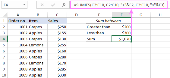
For example, to sum the numbers in the range C2:C10 that are greater than 200 and less than 300, the formula is:
=SUMIFS(C2:C10, C2:C10, ">200", C2:C10, "<300")
To make the formula more flexible, you can input the smallest and largest numbers in predefined cells (F2 and F3 in this example) and reference those cells. In this case, the syntax of the criteria is slightly different: you enclose a logical operator in double quotes and concatenate a cell reference using an ampersand. For example:
=SUMIFS(C2:C10, C2:C10, ">"&F2, C2:C10, "<"&F3)

SUMIF between two values in Excel
The formula works in Excel 2000 - Excel 365
If you have an old version of Excel where the SUMIFS function is not available, then you can emulate the functionality by using its singular counterpart - the SUMIF function.
The idea is to construct two separate SUMIF functions:
- The first one adds up the values greater than the minimal number.
- The other one sums the values greater than or equal to the maximum number.
Then, you subtract the latter from the former and get the desired result.
To make sure the formula works as expected, let's test it on the same dataset:
=SUMIF(C2:C10, ">200") - SUMIF(C2:C10, ">=300")
Or with the cell references:
=SUMIF(C2:C10, ">"&F2) - SUMIF(C2:C10, ">="&F3)

SUMIFS between two numbers with additional criteria
The beauty of the SUMIFS function is that accepts multiple range/criteria pairs (up to 127). Meaning, in the generic SUMIFS formula discussed above, you can include as many different criteria as needed.
For example, to sum the Grapes sales between $200 and $300, the formula takes this form:
=SUMIFS(C2:C10, C2:C10, ">200", C2:C10, "<300", B2:B10, "Grapes")
With cell references, it works equally well:
=SUMIFS(C2:C10, C2:C10, ">"&F3, C2:C10, "<"&F4, B2:B10, F2)

SUMIF between in Google Sheets
The good news is that the SUMIFS formulas we've built for Excel work in Google Sheets too, without a single change in the syntax. Thank you for the consistency, Microsoft and Google! :)
SUMIFS between two numbers
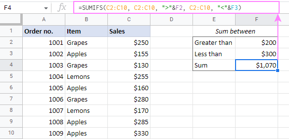
To get a sum of the values in column C that fall in the range between the numbers in F2 and F3, the formula is:
=SUMIFS(C2:C10, C2:C10, ">"&F2, C2:C10, "<"&F3)

SUMIFS between two values with another condition
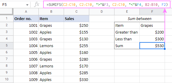
To add up the sales numbers for a specific item in F2 that are between the numbers in F3 and F4, the formula is:
=SUMIFS(C2:C10, C2:C10, ">"&F3, C2:C10, "<"&F4, B2:B10, F2)

That's how to sum data between two values in Excel and Google Sheets. Amazingly simple, isn't it? I thank you for reading and hope to see you on our blog next week!
Practice workbooks
SUMIF between values in Excel (.xlsx file)
SUMIF between numbers in Google Sheets (online sheet)
 by
by
8 comments
100 (T) 200 (T) 300 (C) 100 (C) 100 (T)
What is the formula for adding the T or the total C?
Hi! If this text is written in cell A1, the formula for the conditional sum can be as follows:
=LET(t, TEXTSPLIT(A1," "), r, WRAPROWS(t,2), SUM(FILTER(VALUE(CHOOSECOLS(r,1)), CHOOSECOLS(r,2)="(T)")))
TEXTSPLIT(A1," ") → t
Splits the text in cell A1 by spaces. Read more: TEXTSPLIT function in Excel: split text strings by delimiter.
WRAPROWS(t,2) → r
Rearranges the list into 2 columns (pairs). For the detailed instructions, please see: Convert column / row to array in Excel: WRAPCOLS & WRAPROWS.
CHOOSECOLS(r,1)
Takes the first column = numbers (100, 200, 300, 100, 100). Read: Excel CHOOSECOLS function to get columns from array or range.
CHOOSECOLS(r,2)
Takes the second column = tags ((T), (T), (C), (C), (T)).
FILTER(VALUE(CHOOSECOLS(r,1)), CHOOSECOLS(r,2)="(T)")
Keeps only the numbers where the tag = (T).
Gives {100; 200; 100}.
See an examples: Excel FILTER function - dynamic filtering with formulas.
SUM(...)
SUM function adds them up → 400.
Universal furmula (specify the letter in cell B1: T or C):
=LET(tag, "(" & B1 & ")", t, TEXTSPLIT(A1," "), r, WRAPROWS(t,2), SUM(FILTER(VALUE(CHOOSECOLS(r,1)), CHOOSECOLS(r,2)=tag)))
You can also find useful information in this article: Excel LET function with formula examples
32 +32+3+(28+5) HOW TO SUM TOTAL IN EXCEL
Hi! I recommend reading this guide:How to make formulas in Excel
Hi Team,
In Excel workbook a sheet called A, there is a cell called a1, there is value called 1+2. Now, in the same work book another sheet called B, I want only the value of the first number of the cell a1 if sheet A.
Hi! To extract the number before the "+" sign from a cell, use these guidelines: How to extract text before a specific character. This should solve your task.
i need an excel formula for Average the sales that were made in Amazon and fall under the Toy Category
Hi! To calculate average sales by multiple criteria, use the AVERAGEIFS function.