The tutorial explains how to use COUNTIFS and COUNTIF formulas with multiple criteria in Excel based on AND as well as OR logic. You will find a number of examples for different data types - numbers, dates, text, wildcard characters, non-blank cells and more.
Of all Excel functions, COUNTIFS and COUNTIF are probably most often mixed up because they look very much alike and both are purposed for counting cells based on the specified criteria.
The difference is that COUNTIF is designed for counting cells with a single condition in one range, whereas COUNTIFS can evaluate different criteria in the same or in different ranges. The aim of this tutorial is to demonstrate different approaches and help you choose the most efficient formula for each particular task.
Excel COUNTIFS function - syntax and usage
The Excel COUNTIFS function counts cells across multiple ranges based on one or several conditions. The function is available in Excel 365, 2021, 2019, 2016, 2013, Excel 2010, and Excel 2007, so you can use the below examples in any Excel version.
COUNTIFS syntax
The syntax of the COUNTIFS function is as follows:
- criteria_range1 (required) - defines the first range to which the first condition (criteria1) shall be applied.
- criteria1 (required) - sets the condition in the form of a number, cell reference, text string, expression or another Excel function. The criteria defines which cells shall be counted and can be expressed as 10, "<=32", A6, "sweets".
- [criteria_range2, criteria2]… (optional) - these are additional ranges and their associated criteria. You can specify up to 127 range/criteria pairs in your formulas.
In fact, you don't have to remember the syntax of the COUNTIF function by heart. Microsoft Excel will display the function's arguments as soon as you start typing; the argument you are entering at the moment is highlighted in bold.

Excel COUNTIFS - things to remember!
- You can use the COUNTIFS function in Excel to count cells in a single range with a single condition as well as in multiple ranges with multiple conditions. If the latter, only those cells that meet all of the specified conditions are counted.
- Each additional range must have the same number of rows and columns as the first range (criteria_range1 argument).
- Both contiguous and non-contiguous ranges are allowed.
- If the criteria is a reference to an empty cell, the COUNTIFS function treats it as a zero value (0).
- You can use the wildcard characters in criteria - asterisk (*) and question mark (?). See this example for full details.
How to use COUNTIFS and COUNTIF with multiple criteria in Excel
Below you will find a number of formula examples that demonstrate how to use the COUNTIFS and COUNTIF functions in Excel to evaluate multiple conditions.
How to count cells with multiple criteria (AND logic)
This scenario is the easiest one, since the COUNTIFS function in Excel is designed to count only those cells for which all of the specified conditions are TRUE. We call it the AND logic, because Excel's AND function works this way.
Formula 1. COUNTIFS formula with multiple criteria
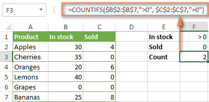
Suppose you have a product list like shown in the screenshot below. You want to get a count of items that are in stock (value in column B is greater than 0) but have not been sold yet (value is column C is equal to 0).
The task can be accomplished by using this formula:
=COUNTIFS(B2:B7,">0", C2:C7,"=0")
And the count is 2 ("Cherries" and "Lemons"):
Formula 2. COUNTIFS formula with two criteria
When you want to count items with identical criteria, you still need to supply each criteria_range / criteria pair individually.
For example, here's the right formula to count items that have 0 both in column B and column C:
=COUNTIFS($B$2:$B$7,"=0", $C$2:$C$7,"=0")
This COUNTIFS formula returns 1 because only "Grapes" have "0" value in both columns.
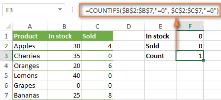
Using a simpler formula with a single criteria_range like COUNTIFS(B2:C7,"=0") would yield a different result - the total count of cells in the range B2:C7 containing a zero (which is 4 in this example).
How to count cells with multiple criteria (OR logic)
As you have seen in the above examples, counting cells that meet all of the specified criteria is easy because the COUNTIFS function is designed to work this way.
But what if you want to count cells for which at least one of the specified conditions is TRUE, i.e. based on the OR logic? Overall, there are two ways to do this - by adding up several COUNTIF formulas or using a SUM COUNTIFS formula with an array constant.
Formula 1. Add up two or more COUNTIF or COUNITFS formulas
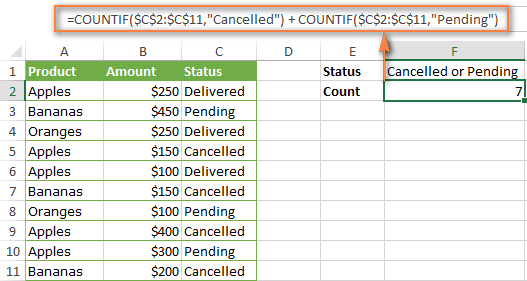
In the table below, supposing you want to count orders with the "Cancelled" and "Pending" status. To have it doen, you can simply write 2 regular Countif formulas and add up the results:
=COUNTIF($C$2:$C$11,"Cancelled") + COUNTIF($C$2:$C$11,"Pending")
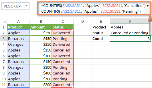
In case each of the functions is supposed to evaluate more than one condition, use COUNTIFS instead of COUNTIF. For example, to get the count of "Cancelled" and "Pending" orders for "Apples" use this formula:
=COUNTIFS($A$2:$A$11, "Apples", $C$2:$C$11,"Cancelled") + COUNTIFS($A$2:$A$11, "Apples", $C$2:$C$11,"Pending")
Formula 2. SUM COUNTIFS with an array constant
In situations when you have to evaluate a lot of criteria, the above approach is not the best way to go because your formula would grow too big in size. To perform the same calculations in a more compact formula, list all of your criteria in an array constant, and supply that array to the criteria argument of the COUNTIFS function. To get the total count, embed COUNTIFS inside the SUM function, like this:
In our sample table, to count orders with the status "Cancelled" or "Pending" or "In transit", the formula would go as follows:
=SUM(COUNTIFS($C$2:$C$11, {"cancelled", "pending", "in transit"}))
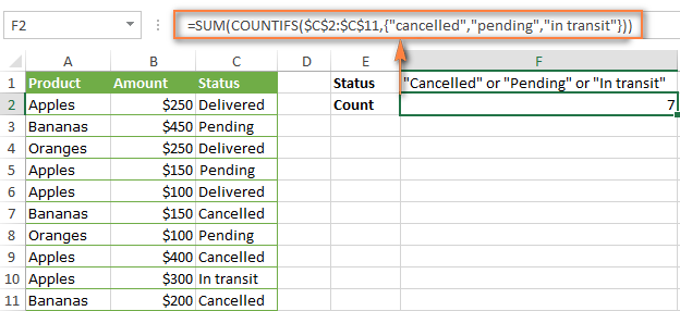
In a similar manner, you can count cells based on two or more criteria_range / criteria pairs. For instance, to get the number of "Apples" orders that are "Cancelled" or "Pending" or "In transit", use this formula:
=SUM(COUNTIFS($A$2:$A$11,"apples",$C$2:$C$11,{"cancelled","pending","in transit"}))

You can find a few more ways to count cells with OR logic in this tutorial: Excel COUNTIF and COUNTIFS with OR conditions.
How to count numbers between 2 specified numbers
By and large, COUNTIFS formulas for numbers fall into 2 categories - based on several conditions (explained in the above examples) and between the two values you specify. The latter can be accomplished in two ways - by using the COUNTIFS function or by subtracting one COUNTIF from another.
Formula 1. COUNTIFS to count cells between two numbers
To find out how many numbers between 5 and 10 (not including 5 and 10) are contained in cells C2 through C10, use this formula:
=COUNTIFS(C2:C10,">5", C2:C10,"<10")
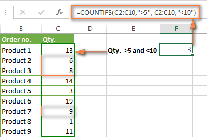
To include 5 and 10 in the count, use the "greater than or equal to" and "less than or equal to" operators:
=COUNTIFS(B2:B10,">=5", B2:B10,"<=10")
Formula 2. COUNTIF formulas to count numbers between X and Y
The same result can be achieved by subtracting one Countif formula from another. The first one counts how many numbers are greater than the lower bound value (5 in this example). The second formula returns the count of numbers that are greater than the upper bound value (10 in this case). The difference between the first and second number is the result you are looking for.
- =COUNTIF(C2:C10,">5")-COUNTIF(C2:C10,">=10") - counts how many numbers greater than 5 and less than 10 are in the range C2:C10. This formula will return the same count as shown in the screenshot above.
- =COUNTIF(C2:C10, ">=5")-COUNTIF(C2:C10, ">10") - the formula counts how many numbers between 5 and 10 are in the range C2:C10, including 5 and 10.
How to use cell references in COUNTIFS formulas
When using logical operators such as ">", "<", "<=" or ">=" together with cell references in your Excel COUNTIFS formulas, remember to enclose the operator in "double quotes" and
add an ampersand (&) before a cell reference to construct a text string.
In a sample dataset below, let's count "Apples" orders with amount greater than $200. With criteria_range1 in cells A2:A11 and criteria_range2 in B2:B11, you can use this formula:
=COUNTIFS($A$2:$A$11, "Apples", $B$2:$B$11, ">200")
Or, you can input your criteria values in certain cells, say F1 and F2, and reference those cells in your formula:
=COUNTIFS($A$2:$A$11, $F$1, $B$2:$B$11, ">"&$F$2)
Please notice the use of absolute cell references both in the criteria and criteria_range arguments, which prevents the formula from being broken when copied to other cells.
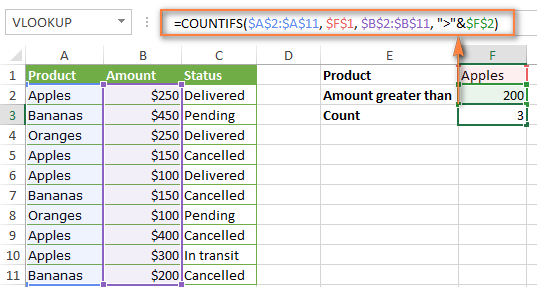
For more information about the use of an ampersand in COUNTIF and COUNTIFS formulas, please see Excel COUNTIF - frequently asked questions.
How to use COUNTIFS with wildcard characters
In Excel COUNTIFS formulas, you can use the following wildcard characters:
- Question mark (?) - matches any single character, use it to count cells starting and/or ending with certain characters.
- Asterisk (*) - matches any sequence of characters, you use it to count cells containing a specified word or a character(s) as part of the cell's contents.
Tip. If you want to count cells with an actual question mark or asterisk, type a tilde (~) before an asterisk or question mark.
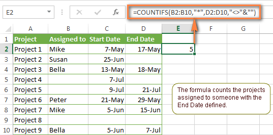
Now let's see how you can use a wildcard char in real-life COUNTIFS formulas in Excel. Suppose, you have a list of projects in column A. You wish to know how many projects are already assigned to someone, i.e. have any name in column B. And because we are learning how to use the COUNTIFS function with multiple criteria, let's add a second condition - the End Date in column D should also be set.
Here is the formula that works a treat:
=COUNTIFS(B2:B10,"*",D2:D10,"<>"&""))
Please note, you cannot use a wildcard character in the 2nd criteria because you have dates rather that text values in column D. That is why, you use the criteria that finds non-blank cells: "<>"&""
COUNTIFS and COUNTIF with multiple criteria for dates
The COUNTIFS and COUNTIF formulas you use for dates are very much similar to the above formulas for numbers.
Example 1. Count dates in a specific date range
To count the dates that fall in a certain date range, you can also use either a COUNTIFS formula with two criteria or a combination of two COUNTIF functions.
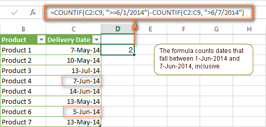
For example, the following formulas count the number of dates in cells C2 through C10 that fall between 1-Jun-2014 and 7-Jun-2014, inclusive:
=COUNTIFS(C2:C9, ">=6/1/2014", C2:C9, "<=6/7/2014")
=COUNTIF(C2:C9, ">=6/1/2014") - COUNTIF(C2:C9, ">6/7/2014")
Example 2. Count dates with multiple conditions
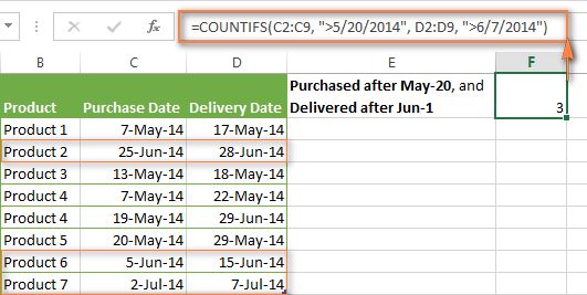
In the same manner, you can use a COUNTIFS formula to count the number of dates in different columns that meet 2 or more conditions. For instance, the below formula will find out how many products were purchased after the 20th of May and delivered after the 1st of June:
=COUNTIFS(C2:C9, ">5/1/2014", D2:D9, ">6/7/2014")
Example 3. Count dates with multiple conditions based on the current date
You can use Excel's TODAY() function in combination with COUNTIF to count dates based on the current date.
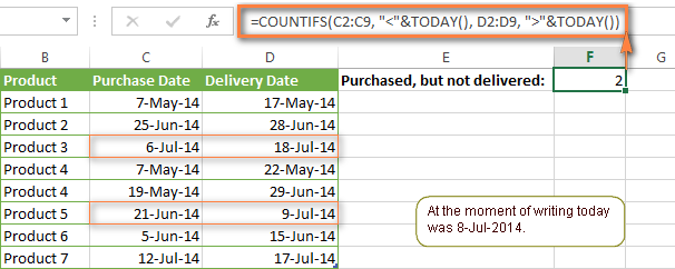
For example, the following COUNTIF formula with two ranges and two criteria will tell you how many products have already been purchased but not delivered yet.
=COUNTIFS(C2:C9, "<"&TODAY(), D2:D9, ">"&TODAY())
This formula allows for many possible variations. For instance, you can tweak it to count how many products were purchased more than a week ago and are not delivered yet:
=COUNTIFS(C2:C9, "<="&TODAY()-7, D2:D9, ">"&TODAY())
This is how you count cells with multiple criteria in Excel. I hope you will find these examples helpful. Anyway, I thank you for reading and hope to see you on our blog next week!
 by
by
1979 comments
Hi there, I am trying to program a workbook to pull data from different sheets and am hitting a roadblock in trying to program my COUNTIFS formula with multiple criteria.
I am pulling survey data and am looking at the number of compliments per city. In this instance, I have it programmed to pull the comment number that are compliments and from the city, but where I am running into trouble is that the city field comes back to me and can reflect the city of North Fort Myers as "NORTH FORT M" and "N FORT MYERS".
I am trying to figure out how I can program it so both of these are picked up for the same total number. I currently have my formula as =COUNTIFS(Test!O:O,List!W2,Test!D:D,List!C2). But for the data in column D, I want it to be pulled if it reflects the info from cells C2 and D2.
Hoping this is clear and you can help! Thanks.
Hi! Unfortunately, the COUNTIFS function cannot calculate approximate matches. To use the formulas, correct the typos. You can use the Find Fuzzy Duplicates tool to do this. It is available as a part of our Ultimate Suite for Excel that you can install in a trial mode and check how it works for free.
Hi Alexander,
I'm trying to use Countifs with Text.
I have a column with Girls attending classes. In that column I write yes or No.
I then would like to calculate or create a formula in a separate column, that if that specific cell says "Yes" it would allow the formula to occur if it says "No" it would just appear as £0.
Hoping you can help me.
Thanks
Is this also possible to occur with a Dropdown with either yes or no? And How would I allow the formula to occur or have it cancel it out if it say no.
Thanks
Hello! I don't really understand what result you want to get. If you want to count the quantity "Yes", use the COUNTIF function: COUNTIF(B2:B10,"Yes")
If you want to calculate a formula by condition, use the IF function.
Hi Alexander,
What would be the formula for the following example:
Column A has three entries "house", "bungalow" or "flat". Column B has the 'area' of the building. I want to calculate the total area when Column A has either "house" or "bungalow" entered.
I hope this makes sense!
Thanks :)
Hi! The following tutorial should help: Excel SUMIFS and SUMIF with multiple criteria – formula examples.
For example,
=SUMIFS(B1:B10,A1:A10,"house") + SUMIFS(B1:B10,A1:A10,"bungalow")
Hi, I am trying to total how many times a participant has attended a class over a 6 week period. I have Column A containing the names of participants, column B containing the date attended. These participants names listed in column A are repeated in alot of cases as they might attend multiple times over this period. I am wanting to lookup column A, find the exact same names/search criteria and return a total "number" for the sum of how many times their name appears over this period. This would then tell me that "Joe Blow" attended this class 20 times over a 6 week period. Thank you. Ruth :-)
Hi! I hope you have studied the recommendations in the tutorial above. It contains answers to your question. Here is an example formula for your case:
=COUNTIFS(A1:A100,"Joe Blow", B1:B100,"<"&TODAY(), B1:B100,">"&(TODAY()-42))
Hi,
I have 2 columns. Column A shows the time and Column B indicates if a button is pushed with 1='button pushed' and 0='button not pushed'. i need to measure the time between every button push (or the number of cells between each '1' because each cell is equal to 1 minute) but the data spans over 2 weeks (=20 000++ cells). is there a way to make a list of the duration for every "downtime" (time between every button push) without doing them one by one?
for example, collumn B would look something like this:
0,0,0,0,0,0,1,0,0,0,0,0,0,0,0,0,0,0,0,0,0,0,0,0,0,0,0,0,0,1,0,0,0,0,0,0,1,0,0,0,0,0,0,0,0,0,0,0,0,0,0,0,0,0,0,1,0,0,....
so the first downtime is 22 minutes, second downtime is 6 minutes, third downtime is 18 minutes and so on.
thanks in advance!
Hi! If I understand your task correctly, the following formula should work for you:
=SEARCH("#",SUBSTITUTE(CONCAT($B$1:$B$3000),"1","#",ROW(A2))) - SEARCH("#",SUBSTITUTE(CONCAT($B$1:$B$3000),"1","#",ROW(A1)))-1
Copy this formula down along the column. I hope this will help.
Thank you so much! it works wonderfully!
I changed the '3000' in '$B$3000' to the number of the final cell.
why do we need to use ROW(A1)? I substituted it with 1,2,3,.... and it work just fine, but your method also work. what is the difference?
If you copy the formula down along the column, the value of ROW(A1) will automatically change and return 1,2,3...
Ok everything is clear now! thanks again!
I need help in my file as per below sample.
I have multiple items, some are with same "PCA P/N" and some are not same and it has different date reject each PCA P/N recorded.
Then, what I need is to count the specific PCA P/N which still "OPEN" status and with less than 30days from now.
Another column and formula is for less than 60 days, and next is less than 90days from now.
For example the Date Reject is at column A:A, PCA P/N is at column B:B and the status is at column C:C.
Date Reject PCA P/N STATUS
5-Aug-22 AEM5300-66402 open
Hope you guys understand my statement.
Hi! If I understand your task correctly, try the following formula:
=SUM(((TODAY()-A1:A20)<30)*(B1:B20="AEM5300-66402")*(C1:C20="open"))
or
=SUMPRODUCT(--((TODAY()-A1:A20)<30),--(B1:B20="AEM5300-66402"),--(C1:C20="open"))
For more information, please visit: Excel SUMPRODUCT function with multiple criteria - formula examples.
Thanks for your response. But after I've tried, this is the results.
for this one -> =SUM(((TODAY()-A1:A20)<30)*(B1:B20="AEM5300-66402")*(C1:C20="open")) results shows "0".
and for the 2nd formula shows #VALUE!.
I'll check on your link provided for more other info.
Thanks again.
I'm checking the error and evaluate the formula shows the date is "45072-A1:A20".What do i need to change or format?
I wrote this formula based on the description you provided in your original comment. I can't see your data and can't know what dates you are comparing. Also check the dates in column A. If it's text and not dates, the formula doesn't work. Please note that if you’d provided me with the precise and detailed description of your task from the very beginning, I’d have created a different formula that would have worked for your case.
Hi Sir,
Appreciated your response and thank you.
Actually the output should be like this.
Model <30 days <60 days <90 days 120 days
M5300-66401 8 3 1 0 3
Everyday it will count those within 30 days from today, those within 60days from today and so on.
Those status still "open", and yes the column A is formatted as date.
By right your formula will work but i don't get it also why having error.
Hi! Your answer does not contain any new data that would help give you advice. Check column A. I think it contains text that is formatted as a date. Pay attention to the following article: How to convert text to date in Excel.
Hi, Please help with the below formula.
The top performer's indication with a yes or no is in column "L". Country is in column X. Now I would like to understand the % of top performers in the United Kingdom and Ireland countries. Used the below formulae but couldn't get the correct %. Please help.
=COUNTIFS('Successors List'!L:L,"Yes",'Successors List'!X:X,"United Kingdom","Ireland")/COUNTIF('Successors List'!L:L,"Yes")
* To clarify, the "Successors list" is the top performers list in the Excel file.
Hi! Pay attention to the following paragraph of the article above: How to count cells with multiple criteria (OR logic).
It covers your case completely.
COUNTIFS('Successors List'!L:L,"Yes",'Successors List'!X:X,"United Kingdom") + COUNTIFS('Successors List'!L:L,"Yes",'Successors List'!X:X,"Ireland")
Hi, Many many thanks for responding. I've used the formula already. However, it shows 3000% which is weird. Do you know why is it not giving the right %?
I can't check your formula because I don't have your data.
Hi!
Would love some formula help here, if possible.
Sheet 1: Customer email (column A), Survey completion date (column B)
Sheet 2: Customer email (column A), Order date (column B), Unique order # (column C)
On Sheet 1 in column C, would like a formula to count quantity of unique orders on Sheet 2 by customer email BEFORE OR ON the survey completion date
Is this something you could help me with?
Hello!
If I understand your task correctly, the following formula should work for you:
=SUM((COUNTIFS('1'!A1:A10,'2'!A1:A10,'1'!B1:B10,">="&'2'!B1:B10)))
Hi Alexander,
I follow your topics and website. You are genius of solving the problems. And you help me many times here.
My question is:
I have one cell A1. Every week in this cell is entering one of this letters ("A", "B", "C","D") from another sheet. . I want to count this letter and multiply by different number.
For Example: countif(A1,"A")*13.75 ........... countif(A1,"D")*2.75 ............ countif(A1,"C")*5.5 ............... countif(A1,"B")*8.25
I want to put this in one formula.
Thank you
Hi! You can get a number depending on the value of the cell using the IFS function.
IFS(A1="A",13.75,A1="B",2.75,A1="C",5.5,A1="D",8.25)
But I'm not understood what result you want to get and why you should use COUNTIF in the one cell.
I thought that I have to use countifs, because i have multiple criterias. Also think about IF with OR. But couldn't put together.
Thank you for quick response.
Result is based on £. For example: if in that cell A1 is D, then I want to be multiplied by 2.75£. People are receiving bonuses for their hard work.
I make setup with your formula IFS and this solve my problem.
Thank you very much.
how can i count total number of unstanding payment for one registration number ( different pay rate) from different worksheet( one worksheet for one month) for the whole year.
Hi! Create a COUNTIFS formula for each sheet separately, and then sum them up.
Maybe this article will be helpful: Excel reference to another sheet or workbook (external reference)
Hi,
Could you please help to solve below problem?
I just need to get the result with count of text from two columns in a particular range whether the values are same for both cells or different in both cells, the values shall be counted as one only.
Example:
A B
Apple Orange
Orange Mango
Apple Orange
Apple 2
Orange 3
Mango 1
Sorry, a change in example:
A B
Apple Apple
Orange Mango
Apple Orange
Apple 2
Orange 2
Mango 1
Hi! To count the number of values by condition, use COUNTIF function and this guide: COUNTIF function in Excel - count if not blank, greater than, duplicate or unique.
For example:
=COUNTIF(A1:B6,"apple")
=SUM(COUNTIFS($A$2:$A$11,"apples",$C$2:$C$11,{"cancelled","pending","in transit"}))
how we write like this
=SUM(COUNTIFS($A$2:$A$11,"apples",$C$2:$C$11,{"="&H1(Like),"="&H2(Like), "="&H3(Like),"="&H4(Like)}))
Hi! Please clarify your specific problem or provide additional details to highlight exactly what you need. As it's currently written, it's hard to tell exactly what you're asking.
Hi
I'm looking at calculating the count of employees who belong to the United Kingdom and Ireland. But I need to calculate just within 4 cells and not more.
The country is in the AF column, and I need to look at the formula calculating no. of employees who are in the UK and Ireland in 2 different time frames.
Used the below formula but is not working. AF52:AF53 is one time frame and AF57:AF58 is another timeframe.
=COUNTIFS(AF52:AF53,"United Kingdom",AF57:AF58,"United Kingdom") + COUNTIFS(AF52:AF53,"Ireland",AF57:AF58,"Ireland")
Please help!!!
Hi! I can't check your formula because I don't have your data. Note, however, that the COUNTIFS function only counts when, for example, AF52=AF57="United Kingdom"
This may help.
=COUNTIFS(AF52:AF53,{"United Kingdom","Ireland"})+COUNTIFS(AF57:AF58,{"United Kingdom","Ireland"})
Hi,
How do copy the formula to another cell with skipping AZ-BA (2 Columns) of data.
=COUNTIFS(AV$6:AV$75,"12x12",AW$6:AW$75,"Prep")+COUNTIFS(AV$6:AV$75,"12x12",AX$6:AX$75,"Prep-c")+COUNTIFS(AV$6:AV$75,"12x12",AY$6:AY$75,"Prep")
into
=COUNTIFS(BB$6:BB$75,"12x12",BC$6:BC$75,"prep")+COUNTIFS(BB$6:BB$75,"12x12",BD$6:BD$75,"Prep")+COUNTIFS(BB$6:BB$75,"12x12",BE$6:BE$75,"prep")
Hi!
I recommend reading this guide: How to copy formula in Excel with or without changing references.
Hi,
I have this table with list of names and 3 columns for the status. The reference is from another sheet. i used countifs with 2 conditions and working except for 2 names, that returns the value of 0. I checked the reference and they should value greater than 0. I tried it also in google sheet and got the same result. Also, tried changing the format but no changes. Hope you can help. Thank you.
The formula is like this
=COUNTIFS(Sheet2!A:A,A2,Sheet2!B:B,B1)
Hope you can help. Thank you.
Can anyone
Hi! I can't check your formula because I don't have your data. It is possible that your values have extra spaces, unprintable characters, or decimals that are hidden by the number formatting.
Hi! I would like to ask about, what formula is the best for this situation:-
COLOUMN A : Name of officer
COLOUMN B : Name of officer
COLOUMN C : Numbers of day taken to complete the task
Reason why there are two column is the task need to 2 officers to be completed. So the question is, how do I want to count if the officer (e.g Lisa) has completed her task less than 7 days.
Thank you.
Hi! You can use the COUNTIFS function to calculate an sum for several conditions. Use this guide: How to use Excel COUNTIFS and COUNTIF with multiple criteria.
It is not possible to give more detailed advice since you have not provided any data.
I need some help! I am an OB provider and in the last 6 years, my male-to-female fetus ratio is 2:1 (which is wild). I am trying to see if the sex discrepancy is the strongest based on specific indications (such as mothers over 35 or patients I saw due to sonogram anomalies). I have my indications (the reason they saw me) in one column and male or female in another column. I use this [COUNTIF(F:F, "(u/s)*")] to indicate patients that were seen due to sonogram anomalies and [COUNTIF(I:I,"*male*")] to indicate all male fetuses.
Can I combine the two and see whether the indication changes the sex ratio?
Hello!
If I understand your question correctly, try using the COUNTIFS function to count values for the two conditions:
COUNTIFS(F:F, "(u/s)*", I:I,"*male*")
Look for the example formulas here: Excel COUNTIFS and COUNTIF with multiple AND / OR criteria.
Hi Alexander!
Thanks for your blog, it's very useful. I had a question, I hope you can help me. I would like to count how many cells in a column contain simultaneously certain words (not just one word, as CTRL+F would be enough). Let me explain better.
I'm doing a list of magazine articles that talk about several topics, I'm classifying them. For example, let's say I have 50 articles, one listed under the other (in 50 rows), and categorized through 4 criteria (columns): theme of the Article (column A), Author (column B), Title (column C), Editor (column D).
The important one is Column A, where I list the topics each of the articles talks about. So in each cell of Column A, for each article, I put certain keywords separated by commas. Example:
column A (Topics present in the article) column B (author) column C (title) column D (editor)
Row/article 1: food, travel, social media, money XXXXX XXXXX XXXXX
Row/article 2: food, money, tourism XXXXX XXXXXX XXXXX
Row/article 3: travel, food, sustainability
Row/article 4: social media, money, travel
Row/article 5: sustainability, food, social media
QUESTION: How many cells of column A contain both "food" and "travel"? Or both "travel" AND "money" AND "food"?
I would like to know many articles talk about several topics at the same time, so how many times certain keywords are mentioned simultaneously within the same cell. For example, how many articles talk about both food and travel (how many cells of column A contain both "food" and "travel")? How many articles talk about both money and social media (how many cells of column A contain both "money" and "social media")? And even three topics simultaneously.
Thanks in advance for your help!
Take care,
Hi!
Find a partial match of the text strings using the SEARCH function.
=SUM(--ISNUMBER(SEARCH("food",A1:A20))*(--ISNUMBER(SEARCH("travel",A1:A20))))
For more information, please read: How to find substring in Excel
Thanks for your answer!
Maybe I didn't understand something because when I try to apply the formula to the desired column it doesn't show the correct results. For example I know for sure at least 5 cells contain simultaneously two certain words, and still the formula tells me only one cell does, or none.
I mean, does it count how many cells IN TOTAL in a certain column contain at least the words used in the formula, or the formula just works for each cell individually? Sorry forr my question, I'm not that familiar with Excel.
Thanks again,
Hi!
The formula counts how many cells in the range contain 2 words at the same time. I can't see your data, but the formula works for me.
Hello there!
Yes, indeed the formula works, thanks! The only issue is the range. Instead of giving me the results for the whole range (like 10 articles in total mentioning X and Y), it only works for individual cells: I have to drag the formula down, in paralel to the column with the keywords I want to count, and it gives a list of results per cell (like 0, 0, "1", 0, 0, "1", 0, "1", etc.), not the total of the range ("3"). I don't understand why.
So I then have to sum the whole column of results to have the total number of articles mentioning the chosen words. It's like the "extracting part" works, indentifying the words, but the "sum part" doesn't for the whole range, only for individual cells.
I could send you a part of the file as an example or screenshots, no problem.
Thanks again!
Dear Alexander,
Sorry to bother again, I think found a SOLUTION, I wanted to let you know in case future users find it useful.
I simply modified your formula a little bit, changing the =sum with =sumproduct. This way it shows the final results for the whole range of interest in a single cell:
=SUMPRODUCT(--ISNUMBER(SEARCH("KEYWORD1",A:A))*(--ISNUMBER(SEARCH("KEYWORD2",A:A))))
Do you think there is a way to see highlighted the results? I mean, not just knowing the number of cells that contain specific keywords, but also knowing which ones in order to find the articles of interest.
Thanks again for your time, it's incredible how helpful you are and I definetively save this page.
Have a nice day!
Hi! To get cell values that contain specific keywords, you can use the FILTER function. The following tutorial should help: Excel FILTER function - dynamic filtering with formulas.
Hi,
I wonder if you could help me. I have table need to find the correct formula to use,
i want to count the duplicate with multiple creteria.
example :
time date customer Flavour number invoice
2:43 am 07/04/2023 linda jitsu 123
2:44 am 07/04/2023 linda Belt 456
2:45 am 07/04/2023 Henry Belt 789
2:45 am 07/04/2023 Henry Belt 897
2:45 am 07/04/2023 Henry jitsu 456
2:46 am 07/04/2023 Henry Belt 789
how we use countif for flavour Jitsu will show duplicate if more than 1 time entry and for flovour Belt will show duplicate if more than 3 times entry?
Hoping for your help in this matter .
Thank you very much
Best Regards
Hi!
If you want to show products that meet more than 3 times, try the methods suggested in this guide: How to find duplicates in Excel.
For example:
=IF(COUNTIF($D$2:$D$8, $D2)>3, "Duplicate", "")
Hi, I have 2 different set of list boxes 1) Overall, Ops, Apps 2) Overall, CR, BF, AT
KPI Oct-22
TTM 0
As mentioned in the above, i would like to calculate TTM count using above list box combinations. Could you please help
Have you experimented with the suggested techniques in the blog post? If they weren't effective, please provide me with more details about your task, and I'll do my best to recommend a solution.
I'm working on a spreadsheet where the COUNTIF formula was pulling from a local desktop so the formula is now giving me a "REF" error since that employee is no longer here. I can see where I can change the path of the formula but unsure what Table2[#Data],"Administration" is coming from. As I don't see any tables to reference on that report when generated.
=COUNTIF('C:\Users\employee\Downloads\NewHireReport (20).xlsx'!Table2[#Data], "Administration")
If you don't know what Table2[#Data],"Administration" is coming from, how should I know?
I need your help on how the countif/s formula can help me with the sample data below:
OMNIS ID Eval Type Week Day RPID Score Opportunity Opportunity Opportunity
CCADA Regular Eval Week 1 Monday 10545125 90.00% 4.2 COMPLETE STATUS NOTES
CCADA Regular Eval Week 1 Monday 10546620 100.00%
CCADA Regular Eval Week 1 Monday 10544879 100.00%
CLSAN Regular Eval Week 1 Monday 10548087 90.00% 4.2 COMPLETE STATUS NOTES
CLSAN Regular Eval Week 1 Monday 10548155 90.00% 4.2 COMPLETE STATUS NOTES
CLSAN Regular Eval Week 1 Monday 10548052 100.00%
I have this sample data and I wanted to count the column of opportunities (3 dedicated columns) per OMINS ID per week. I tried the countifs formula but I am unsuccessful. I hope you can help me. :)
Your explanation makes it hard for me to understand what you want to calculate. I'll try to guess that you need to calculate the quantity by two criteria.
=COUNTIFS(A2:A10,"CCADA",C2:C10,"Week 1",E2:E10,"<>"&"",F2:F10,"<>"&"",G2:G10,"<>"&"")
If that's not what you want, please tell me exactly what result you want.
I tried to recreate the formula but was still unsuccessful :( I made a simple data below.
Sample Data:
NAME Week Opportunity
Ken Week 1 1.1 Use of Available Resources
Ken Week 1 3.1 File Delivery
Ken Week 1 1.1 Use of Available Resources
Ken Week 2 4.2 Complete Notes
Ken Week 2 4.2 Complete Notes
Ken Week 2 4.1 Action Taken
I would like to see how much Ken did incur the opportunity "1.1 Use of Available Resources" on week 1. Same outcome/principle if I want to see the number of opportunities "4.2 Complete Notes" were incurred on week 2.
I hope this helps and I really thank you for helping me :)
Hi!
I recommended you a formula in which you can specify all the necessary conditions. For example:
=COUNTIFS(A2:A10,"CCADA",C2:C10,"Week 2",E2:E10,"="&"4.2 Complete Notes",F2:F10,"<>"&"",G2:G10,"<>"&"")
I was able to recreate the formula. Thank you so much for the help :)
Hi,
I have a formula =COUNT(IF(MONTH($M:$M)=4,1)) which returns how many dates in a column are in each month (April in the example). However I want to combine this with a search in another column "=Yes". But when I am using COUNTIFS I am getting an error. So in essence I want to calculate how many lines are 'Month' and 'Yes' (where the month is currently dd/mm/yyyy). Any advice greatly received
Hello!
The COUNTIFS function cannot have only a cell value as an argument, but not a formula. Therefore, use the SUMPRODUCT function to calculate values with calculations.
If I understand your task correctly, try the following formula:
=SUMPRODUCT(--(MONTH(M1:M10)=4),--(N1:N10="yes"))
Thank you, however I am coming up with #value!. I believe this maybe because not all the values in column M are dates. The column is linked to arrival dates and if the goods have arrived the cell states 'here'. Can I adapt the formula above to state sumproduct IF cell is date (month = 4) and column N =yes?
Hi!
To ignore errors, replace them with 0 using IFERROR function.
=SUMPRODUCT(--IFERROR(MONTH(M1:M10)=4,0),--(N1:N10="yes"))
Thank you, worked perfectly :-)
Hi,
There is my problem, it's a parking case, I have to know how in a one hour range how many cars arrive in the parking,how many leave and how many are on the parking.
I have my Data table there is an exemple :
Park_Time_IN Park_Time_OUT
01/02/2022 18:54 01/02/2022 19:55
02/02/2022 06:34 02/02/2022 08:21
02/02/2022 07:06 02/02/2022 08:15
And I have my Calendar table, for this period it will be :
Date_Time_A Date_Time_B Departure_Number Arrival_Number Number_Car_in_parking
01/02/2022 18:00 01/02/2022 18:59 ???? ???? ????
01/02/2022 19:00 01/02/2022 19:59
01/02/2022 20:00 01/02/2022 20:59
01/02/2022 21:00 01/02/2022 21:59
01/02/2022 22:00 01/02/2022 22:59
01/02/2022 23:00 01/02/2022 23:59
02/02/2022 00:00 02/02/2022 00:59
02/02/2022 01:00 02/02/2022 01:59
02/02/2022 02:00 02/02/2022 02:59
02/02/2022 03:00 02/02/2022 03:59
02/02/2022 04:00 02/02/2022 04:59
02/02/2022 05:00 02/02/2022 05:59
02/02/2022 06:00 02/02/2022 06:59
02/02/2022 07:00 02/02/2022 07:59
02/02/2022 08:00 02/02/2022 08:59
All my cells have the format : Custom : dd/mm/yyyy hh:mm:ss
I tried many formulas with countif but I didn't have a good result. Do you know which formula should I put?
And also should I seperate in new columns Date and Time cause I don't know if I can easily comparate cells with date&time in it.
Thanks a lot for your help
Hi!
If I understand your task correctly, the following formula should work for you:
arrive -
=COUNTIFS(A1:A10,">="&T1,A1:A10,"<="&T2)
on the parking -
=COUNTIFS(A1:A10,"<="&T1,B1:B10,">="&T2)
T1 and T2 - time
I hope it’ll be helpful.
I need to be able to check if the cell is blank. If it's not, then check the cell for specific text. If that cell is blank, I need to check a separate cell for the same text. Any suggestions on how to do that?
Example in words, if cell A is not blank, check cell A for "apples", if A is blank, go to cell C and check for "apples".
I forgot to say, I'm checking a cell range: i.e. A2:A50 or C2:C50
Hi!
Try to use the recommendations described in this article: Excel Nested IF statements - examples, best practices and alternatives. If I understand your task correctly, try the following formula:
=IF(NOT(ISBLANK(A3)),A3="apples",IF(NOT(ISBLANK(C3)),C3="apples",""))
Hello Sir,
I have some data that is grouped but I just want to use Countif formula on specific columns out of all the columns in grouped data, however i can't ungroup the data and use the formula. Is there any way i can use countif formula to do the same?
Hi, looking to use countifs to help with a roster I'm working on. Column C = days of the week, I want the formula to count all cells containing the initials 'RT' in columns F-J if the corresponding row in column C = Friday. Have read the article above, and am trying this: =COUNTIFS($C$4:$C$49,"Friday", $F$4:J$49,"RT") but getting a #VALUE error. Would really appreciate any help, I'm not very good on Excel
Hello!
The COUNTIFS function can only use ranges of the same size. Your data ranges have different dimensions. So use the SUM function to calculate cells where both conditions are met.
Try this formula:
=SUM(($C$4:$C$49="Friday")*($F$4:J$49= "RT"))
That worked, thankyou soooo much :-)
Hello,
I need help developing a formula.
I have one column with names such as Sarah, William etc between G2:G100. And a seperate column with multiple options such as completed, pending, not completed between I2:I100.
I want to count specifically for an employee (Sarah G2:G100) who has the following answers in I2:I100 "completed" or "pending" or "blank cell" but not count the other answers.
Tried many different formulas. Can you help?
Hi!
Try the formulas described in the article above.
For example,
=COUNTIFS(G2:G100,"Sarah",I2:I100,"completed") + COUNTIFS(G2:G100,"Sarah",I2:I100,"pending")
Hi ,i am looking for a formula helps me to count how many cells in row contains values in a special range,lets say i have a column with the values 6.24 ; 6.8; 7.24; 7.35; 7.24. How can i count the values that are from 6.0 to 6.9 and how many are from 7.0 to 7.45?
Hi!
Please re-check the article above since it covers your case.
=COUNTIFS(A1:A10,">6",A1:A10,"<6.9")
I need to know how many cells in two columns meet certain criteria together. So, for BA3:BA141, ">120" and BB3:BB141, ">80", how do I get the total cells where both those critera are met? So far when I've tried, I get the count of all cells meeting one or the other added up and I need the count of the cells where both are met
Hi!
If I understand your question correctly, use the COUNTIFS function as recommended in the article above.
=COUNTIFS(BA3:BA141, ">120", BB3:BB141, ">80")
Dear Sir
I have two columns , one column have open or closed and other column have S or L. I need formula to count open only with L
OPEN S
CLOSED S
OPEN L
OPEN L
CLOSED L
OPEN S
OPEN L
CLOSED L
OPEN L
Hi!
Use the COUNTIFS function as described in the article above. For an example, see Formula 2.
HI can you help me, the formula when someone chooses one option in the data validation, for example THEORETICAL COURSE, OR PRACTICAL COURSE and automaticallly counts +1 as a student , in the number of students
Hi! Have you tried the ways described in this blog post? If they don’t work for you, then please describe your task in detail, I’ll try to suggest a solution.
I'm creating a list that has 3 sets of criteria, My formula below works fine when "Reference!$E$21" is just one value, but the column has 3 values, and I want to exclude 1.
For example, Reference!$E$21 equals A, and the other two values are T and L. I want to keep the values equal to A and L and exclude T . what is the best way to exclude that value in the formula below?
=IFERROR(IF(Reference!$C$1="H",INDEX('[Data!$A$3:$BR$50000,SMALL(IF(COUNTIFS(Reference!$B$16,'[Data!$U$3:$U$50000,Reference!$B$18,'[Data!$U$3:$U$50000,Reference!$E$21,'[Data!$AM$3:$AM$50000),ROW('[Data!$B$3:$B$50000)-MIN(ROW('[Data!$A$3:$BR$50000))+1),ROW(B1)),COLUMN(B1)),INDEX('[Data!$A$3:$BR$50000,SMALL(IF(COUNTIFS(Reference!$B$16,'[Data!$U$3:$U$50000,Reference!$B$19,'[Data!$U$3:$U$50000,Reference!$E$21,'[Data!$AM$3:$AM$50000),ROW('[Data!$B$3:$B$50000)-MIN(ROW('[Data!$A$3:$BR$50000))+1),ROW(B1)),COLUMN(B1))),"")
Hi!
It is very difficult to understand a formula that contains unique references to your workbook worksheets. Hence, I cannot check its work, sorry.
Hi There,
I'm looking to find a formula that takes Column A (Date) from sheet 2022-2023 + anything in Column H that contains a word (could have other words in it as well) from sheet 2022-2023 and counts it in a cell on another sheet. so basically Column A equals a certain date and if it meets that criteria, count the number of cells in column H that contains that certain word (plus could have other words in the cell)
The closest I have to this is =SUMPRODUCT(--('2022-2023'!A:A=DATE(2023, 1,31)),--('2022-2023'!H:H="Leaders")) but its only counting the exact text where some other cells have "Leaders, Supervisors" and it won't include it.
I've tried this too but getting an Error =COUNTIFS('2022-2023'!A:A,DATE(2023, 1,31),('2022-2023'!H:H,"Leaders"))
Thanks for the help!
Hello!
You can determine a partial match of a word and a text string with the combination ISNUMBER + SEARCH functions.
=ISNUMBER(SEARCH("Leaders",H1:H10))
I hope this will help, otherwise don't hesitate to ask.
Hi there,
It didn't quite work as I'm not looking for a true/false response but more so how many cells contain that word. so for example if there are ten cells in the A column that have the same date, how many of those ten cells in the H column contain the word leaders
Hi!
This works great if you apply it to your SUMPRODUCT formula.
For example,
=SUMPRODUCT(--('2022-2023'!A:A=DATE(2023, 1,31)),--(ISNUMBER(SEARCH("Leaders",'2022-2023'!H:H))))
I can't check the formula that contains unique references to your workbook worksheets.
Hello, the following formula counts the number of times names from a range of cells get listed.
=SUMPRODUCT(8*ISNUMBER(SEARCH(B51,$C$18:$P$41)))
Is there a way to ad a seperate individual cell to the formula to be counted along with the existing range? The individual cell is N4
Hi!
If I understand your task correctly, try the following formula:
=SUMPRODUCT(8*ISNUMBER(SEARCH(B51,$C$18:$P$41)))+(1*ISNUMBER(SEARCH(B51,N4)))
You are awesome....I just had to change N4 to $N$4 and it worked great.
=SUMPRODUCT(8*ISNUMBER(SEARCH(B51,$C$18:$P$41)))+(1*ISNUMBER(SEARCH(B51,$N$4)))
Thank You so much!
I'm sorry. For example, I have a Test A and Test B for Standard 1, as well as Standards 2 and 3. I want the Google Sheet to average the highest score from each standard. For some students, this could be the score on Test A and for others it could be the score on Test B. Is there a way to have the function select the highest of two cells and average it with other cells?
I am looking for a formula that can count the highest of two columns only if the value is above 59. I have been trying different versions of COUNTIFS, but it always ends up counting all of the values that are above 59 instead of only counting the higher one if it is above 59. Is there a way to do this? I am trying to count the highest of two test grades only if it is above a 59.
This is the last thing I tried.
=COUNTIFS(B2>C2,[B2>59])+COUNTIFS(B259])
Thank you for offering your knowledge.
Hi!
As it's currently written, it's hard to tell exactly what you're asking. What result do you want to get? Give an example of the source data and the expected result.
Hi... I have a data where in one column there is a request I'd and on the other column there is a description of activity, e.g. updation of Address, Name, Swift, Postal etc. I want to count the occurance of unique activity with reference to request I'd. Though if there are 4 similar request I'd and activity description against it is updation of Address for 4 times in a row but I have to count them as 1 if all 4 has criteria address into it. So even if the count is 4. I want a formula to count it as 1 only. That means the order entry person worked on the same request 4 times will be considered as 1 request, but if there are other activity against the same req id, it should also show 1 count for it as well. but if the occurance of another activity is more than one it should restrict the count as 1 only.
Kindly help with your expertise
Hello!
The answer to your question can be found in this article: Count unique values with criteria. I hope it’ll be helpful. If something is still unclear, please feel free to ask.
Hi!
What if I need to know if a certain number is between 10% above or below another?
Example:
Seller A price: 100 | Seller B price: 110 = Seller A's price inside of 10% of seller B's price
Is this possible with countif?
Hello!
The COUNTIF function cannot use formulas inside itself. So try the function SUMPRODUCT :
=SUMPRODUCT(--(B1:B5/A1:A5<=1.1))
Hi i have a report that has 8 sheets(by Names) which has a table of contents that i need to count based individual text. However with the countif formula, it came out as date (I.E. 1/0/1900)
Formula as follows
=COUNTIFS(Joel!F4:F25,"NICF019")+COUNTIF(Ivan!F4:F25,"NICF019")+COUNTIF(Amanda!F4:F25,"NICF019")+COUNTIF('Wai Loon'!F4:F25,"NICF019")+COUNTIF('Zu Yang'!F4:F25,"NICF019")+COUNTIF(Elly!F2:F25,"NICF019")+COUNTIF(Hazel!F4:F25,"NICF019")+COUNTIF(Kenneth!F4:F25,"NICF019")
Is the formula incorrect?
Hi! To see a number instead of a date, change the cell format to General. I can't check a formula that contains unique references to the data in your worksheets.
This works well. My formula is okay. Have change the cell to general. :D
Million Thanks
Hello,
I have a spreadsheet where I log employee names for each day of the week, which I select from a dropdown list in each cell. Naturally there is more than one employee working some days, so I used visual basic which allowed me to list multiple variables inside the same cell. However, the cells with the multiple names are not being counted. My current formula is =COUNTIFS(C18:P41,B51:B71)
Is there a formula that will allow me to also count the data in cells that have more than one name listed?
Hello!
Give me an example of the data of how several names are written in a cell, and what separators are used between them. Then I'll try to give some advice.
The data is just names separated by a forward slash as the delimiter. Ex. John Doe / Tim Hobbs in one cell, and Jeffrey Beckham in another.
Currently John Doe & Tim Hobbs aren't being counted,
Hi!
To find a partial match of two text strings, use the function SEARCH.
For example,
=SUMPRODUCT(--ISNUMBER(SEARCH(H1,$A$1:$D$10))
This did something totally unexpected to the totals inside my table where all the name counts were the same. Almost like it added them all together. I wanted them to be counted individually, even if they are in the same cell.
Hi!
To understand what you want to do, give an example of the source data and the desired result.
For example: I need names from my table to be counted each time one appears on my spreadsheet range as shown.
Cell 1 Cell 2 Cell 3 Cell 4 Cell 5
Tremayne 1 Tremayne Joe Fred Richard Richard / Mathew / Joe
Richard 4
Mathew 2 Cell 6 Cell 7 Cell 8 Cell 9 Cell 10
Joe 3 Tony / Erick Darrel / Joe Darrel Richard / Mathew Richard
Darrel 2
Fred 1
Currently the Cells 5, 6, 7, & 9 are not being recognized because they contain more than one name separated by a forward slash.
Hi!
As I recommended earlier, enter the desired name in cell H1 and the formula will show you how many times that name is written in the range on the text lines.
=SUMPRODUCT(--ISNUMBER(SEARCH(H1,$A$1:$D$10)))
You can get a list of all the names if you split text into separate cells and use the UNIQUE function.
I have a project where I have a consistent range, and am trying to eliminate 10 criteria with wildcard text. i.e.:
=COUNTIFS($H:$H,"$W$8",$K:$K,{
"*"&$W$16&"*","*"&$W$17&"*","*"&$W$18&"*","*"&$W$20&"*","*"&$W$21&"*","*"&$W$22&"*","*"&$W$23&"*","*"&$W$24&"*","*"&$W$25&"*","*"&$W$26&"*"})
I realise without my workbook you cannot comment on specifics, but I will be able to extrapolate from working with your produce example.
In your example,
=SUM(COUNTIFS($A$2:$A$11,"apples",$C$2:$C$11,{"cancelled","pending","in transit"}))
the formula returns "3".
My version would be trying to find instances where Apples are not cancelled not pending not in transit, which I expect would return "2".
I cannot just count "delivered" instead, because I am trying to ascertain the number of 'anything that isn't listed'. (I am actually trying to find # "not in transit not cancelled not pending not delivered", in this example, the result would be "0").
I cannot subtract the sum from the total because this produces a negative number (e.g. if someone included both "in transit" and "pending" in the same cell);
I don't want to SUM a series of results, because they'd cancel each other out;
there are no PRODUCTS to calculate because I'm dealing with text.
But I'm also not sure a normal COUNTIFS (even with an array) would be the best way to do it
All of my "" appears not to have shown in the original post.
Just to reiterate, the array of 'criteria 2' in my formula need to be NOT"*"&$W$16&"*", NOT"*"&$W$17&"*", etc because I am trying to eliminate these ten categories
Hello!
If I understand your task correctly, the following formula should work for you:
=COUNTIFS($A$2:$A$11,"apples") - SUM(COUNTIFS($A$2:$A$11,"apples",$C$2:$C$11,{"cancelled","pending","in transit"}))
Hi,
I have two check boxes in a single cell. I know the simple COUNTIF formula for counting the number of checked boxes when there's only one check box option in each cell. However, I can't figure out how to do it for cells with multiple checkboxes within them. Eg. in column G rows 2 and 3 - if someone wants to check Jan in row 2 and leave Feb blank, and then in row 3 Jan is checked but Feb is blank, this would be 1 each for Jan and Feb when totaled up... but what formula can I use to tally them up?
Any help would be much appreciated. Thank you
Hi!
The checkbox returns the value TRUE or FALSE in cell G2. Read more about it here: How to insert checkbox in Excel. Use the value of cell H2 in the COUNTIF formula, in which the formula will be written, for example =IF(G2=TRUE,DATE(2023,1,1),"")
I hope it’ll be helpful.
Thanks for your reply.
May I ask,
What if I have two checkboxes in the same cell, one option being AM and another being PM. How can I tally up the number of checked boxes for each option? Eg, In G2 the AM checkbox is checked and PM is unchecked, whilst in G3 the PM box is checked and AM is unchecked ... meaning the totals are AM 1 and PM 1. Which formula can I use to show these totals?
Really appreciate any help.
Thank you
Hi!
Two checkboxes in the same cell cannot have different values. What you're talking about are checkboxes in two different cells.
Hi, am trying to build a staff rota, and want to tally the number of full weekends off eg sat Day off Sunday off.
I can count all the days off, but I want to count only I'd they both cells say day off. So if both cells say day off it will count as 1 total. Hope that makes sence
Hi!
If your data is written in columns D and E, then you can check the condition for two rows at once using the OFFSET function.
=SUM((D1:D26="saturday")*(OFFSET(D1:D26,1,0)="sunday") * (E1:E26="off")*(OFFSET(E1:E26,1,0)="off"))
For more information, please visit: Excel OFFSET function - formula examples and uses.
Hi,
I have two check boxes in a single cell. I know the simple COUNTIF formula for counting the number of checked boxes when there's only one check box option in each cell. However, I can't figure out how to do it for cells with multiple checkboxes within them. Eg. in column G rows 2 and 3 - if someone wants to check Jan in row 2 and leave Feb blank, and then in row 3 Jan is checked but Feb is blank, this would be 1 each for Jan and Feb when totaled up... but what formula can I use to tally them up?
Any help would be much appreciated. Thank you
I'm struggling to make my countifs work.
I'm using the following formula, and it's giving a zero result when I know it should be a 1
=COUNTIFS('January 2023'!A10:A100,"C38",'January 2023'!C10:C100,"Yes")
"C38" is what I want it to look up (a name) and January 2023 is the sheet with the raw date that needs to be displayed.
I'm trying to find out how many times a particular name has been marked "yes" in January.
is there something I'm missing?
Thanks
Hi!
If you want to find the value in cell C38, don't use quotation marks.
=COUNTIFS('January 2023'!A10:A100,C38,'January 2023'!C10:C100,"Yes")
I hope it’ll be helpful.
It worked!
Thank you so much for your help!
What if I have multiple columns to pull from with the same criteria and I need to add the sum? I'm confused do I still use the add countifs and just change coumns?
Hi!
Have you tried the ways described in this blog post? If they don’t work for you, then please describe your task in detail, I’ll try to suggest a solution.
I hope you can help. I work on chevy cars. occasionally i work on a non chevy car. I am trying to count the number of cars I have worked on in a column that do not match the chevy cars listed in another column. I have this formula but it is counting the blank rows of cars i have yet to work on. =SUMPRODUCT(--(ISNA(MATCH(E3:E200,N3:N20,0))))
This is the formula i am using for counting cars that are chevys. =COUNTIF(E:E,N19) (N19 being a Tahoe)
Trying to change that to not equals () an array (N3:N20) just gets me an error.
Thanks for your help.
Hello!
If I understand your task correctly, try the following formula:
=SUM(--((IFNA(MATCH(E1:E2000,N3:N20,0)+1,1)*(--NOT(ISBLANK(E1:E2000))))=1))
Thanks for your help, that works great!
Good morning,
apologies if already covered and missed but i would greatly appreciate your help to formulate the below:
Count/sum if:
Column A = X
Column B = Y
Between dates 01/01/2023 & 31/01/2023
I can get the first two, getting the count/sum of the cells that meet the two conditions but struggling to get the date range factored in as well
Apologies, the variation on this I am struggling with is also:
Count/sum if:
Column A = X
Column B = Y
if Column C = a January date
Hi!
To calculate the sum by conditions, read carefully this guide: Excel SUMIFS and SUMIF with multiple criteria – formula examples. You can also find useful information in this article: How to use Excel SUMIF with dates.
I hope it’ll be helpful.
Hi, I would like to ask for advice. I am currently working on a database. Is there any formula that can help me count the number of entries in a range of cell?
Example:
Employee X has scheduled leave dates 10, 15, 23 for January and 5, 9 for February and so on for the whole year(considering each month are separate columns)
I would like to count the total number of days Employee X have for the whole year.
Thank you so much in advance!
Hello!
If the column contains the number of vacation days, use the SUMIFS function to calculate the sum of days for an individual employee. If each vacation day is specified separately, count the number of days using the COUNTIFS function.
I hope I answered your question. If something is still unclear, please feel free to ask.
=COUNTIFS(LeadSource, "Google (Not Ad.)",SignedUp,"yes",Calendly!AG2:AG14,>="08/01/2022)",Calendly!AG2:AG14,>="08/14/2022)")
How to count multiple criteria in a given set of range
Hi!
It is very difficult to understand a formula that contains unique references to your workbook worksheets. Please re-check the article above since it covers your task.