The tutorial explains the basics of Excel format for number, text, currency, percentage, accounting number, scientific notation, and more. Also, it demonstrate quick ways to format cells in all versions of Excel 365, 2021, 2019, 2016, 2013, 2010, 2007 and lower.
When it comes to formatting cells in Excel, most users know how to apply basic text and numeric formats. But do you know how to display the required number of decimal places or a certain currency symbol, and how to apply just the right scientific notation or accounting number format? And do you know the Excel number format shortcuts to apply the desired formatting in a click?
Excel Format basics
By default, all cells in Microsoft Excel worksheets are formatted with the General format. With the default formatting, anything you input into a cell is usually left as-is and displayed as typed.
In some cases, Excel may not display the cell value exactly as you've entered it, though the cell format is left as General. For example, if you type a large number is a narrow column, Excel might display it in the Scientific notation format, something like 2.5E+07. But if you view the number in the formula bar, you will see the original number that you entered (25000000).
There are situations when Excel may automatically change the General format to something else based on the value you input in a cell. For example, if you type 1/4/2016 or 1/4, Excel will treat it as a date and change the cell format accordingly.
A quick way to check the format applied to a certain cell is select the cell and look at the Number Format box on the Home tab, in the Number group:

An important thing to remember is that formatting cells in Excel changes only the appearance, or visual representation, of a cell value but not the value itself.
For example, if you have number 0.5678 in some cell and you format that cell to display only 2 decimal places, the number will appear as 0.57. But the underlying value won't change, and Excel will use the original value (0.5678) in all calculations.
Similarly, you can change the display representation of date and time values the way you want, but Excel will keep the original value (serial numbers for dates and decimal fractions for times) and use those values in all Date and Time functions and other formulas.
To see the underlying value behind the number format, select a cell and look at the formula bar:

How to format cells in Excel
Whenever you want to modify the appearance of a number or date, display cell borders, change text alignment and orientation, or make any other formatting changes, the Format Cells dialog is the main feature to use. And because it the most used feature to format cells in Excel, Microsoft has made it accessible in a variety of ways.
4 ways to open the Format Cells dialog
To change formatting of a certain cell or a block of cells, select the cell(s) you wish to format, and do any of the following:
- Press Ctrl + 1 shortcut.
- Right click the cell (or press Shift+F10), and select Format Cells… from the pop-up menu.

- Click the Dialog Box Launcher arrow at the bottom right corner of the Number, Alignment or Font group to open the corresponding tab of the Format Cells dialog:

- On the Home tab, in the Cells group, click the Format button, and then click Format Cells…

The Format Cells dialog will show up, and you can start formatting the selected cell(s) by using various options on any of the six tabs.
Format Cells dialog in Excel
The Format Cells dialog window has six tabs that provide different formatting options for the selected cells. To find more about each tab, click on the corresponding link:
Number tab - apply a specific format to numeric values
Use this tab to apply the desired format in terms of number, date, currency, time, percentage, fraction, scientific notation, accounting number format or text. The available formatting options vary depending on the selected Category.
Excel Number format
For numbers, you can change the following options:
- How many decimal places to display.
- Show or hide the thousands separator.
- Specific format for negative numbers.
By default, the Excel Number format aligns values right in cells.
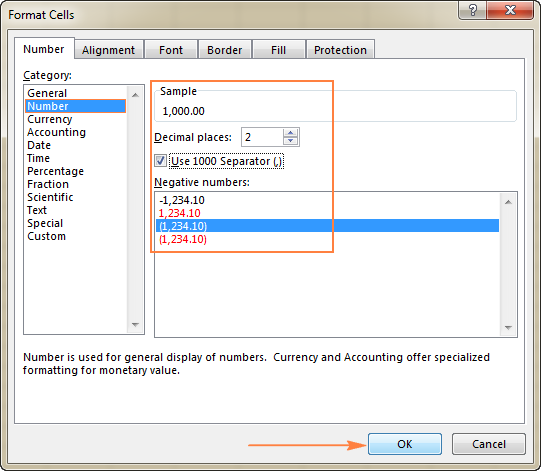
Tip. Under Sample, you can view a life preview of how the number will be formatted on the sheet.
Currency and Accounting formats
The Currency format lets you configure the following three options:
- The number of decimal places to display
- The currency symbol to use
- The format to apply to negative numbers
Tip. To quickly apply the default currency format with 2 decimal places, select the cell or range of cells and press the Ctrl+Shift+$ shortcut.
The Excel Accounting format provides only the first two of the above options, negative numbers are always displayed in parentheses:

Both Currency and Accounting formats are used to display monetary values. The difference is as follows:
- The Excel Currency format places the currency symbol immediately before the first digit in the cell.
- The Excel Accounting number format aligns the currency symbol on the left and the values on the right, zeros as displayed as dashes.

Tip. Some of the most often used Accounting format options are also available on the ribbon. For more details, please see Accounting format options on the ribbon.
Date and Time formats
Microsoft Excel provides a variety of predefined Date and Time formats for different locales:
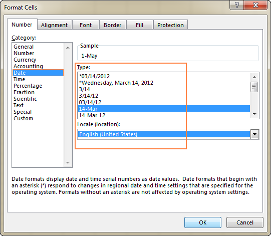
For more information and the detailed guidance about how to create custom date and time format in Excel, please see:
Percentage format
The Percentage format displays the cell value with a percent symbol. The only option that you can change is the number of decimal places.
To quickly apply the Percentage format with no decimal places, use the Ctrl+Shift+% shortcut.
Note. If you apply the Percentage format to the existing numbers, the numbers will be multiplied by 100.
For more information, please see How to show percentages in Excel.
Fraction format
This format lets you choose from a variety of the built-in fraction styles:
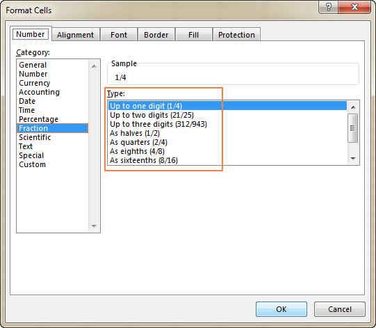
Note. When typing a fraction in a cell that is not formatted as Fraction, you may have to type a zero and a space before the fractional part. For example, if you type 1/8 is a cell formatted as General, Excel will convert it to a date (08-Jan). To input the fraction, type 0 1/8 in the cell.
Scientific format
The Scientific format (also referred to as Standard or Standard Index form ) is a compact way to display very large or very small numbers. It is commonly used by mathematicians, engineers, and scientists.
For example, instead of writing 0.0000000012, you can write 1.2 x 10⁻⁹. And if you apply the Excel Scientific notation format to the cell containing 0.0000000012, the number will be displayed as 1.2E-09.
When using the Scientific notation format in Excel, the only option that you can set is the number of decimal places:

To quickly apply the default Excel Scientific notation format with 2 decimal places, press Ctrl+Shift+^ on the keyboard.
Excel Text format
When a cell is formatted as Text, Excel will treat the cell value as a text string, even if you input a number or date. By default, the Excel Text format aligns values left in a cell. When applying the Text format to selected cells via the Format Cells dialog window, there is no option to be changed.
Please keep in mind that the Excel Text format applied to numbers or dates prevents them from being used in Excel functions and calculations. Numerical values formatted as text force little green triangle to appear in the top-left corner of the cells indicating that something might be wrong with the cell format. And if your seemingly correct Excel formula is not working or returning a wrong result, one of the first things to check is numbers formatted as text.
To fix text-numbers, setting the cell format to General or Number is not sufficient. The easiest way to convert text to number is select the problematic cell(s), click the warning sign that appears, and then click Convert to Number in the pop-up menu. A few other methods are described in How to convert text-formatted digits to number.
Special format
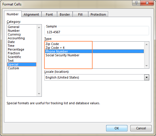
The Special format lets you display numbers in the format customary for zip codes, phone numbers and social security numbers:
Custom format
If none of the inbuilt formats displays the data the way you want, you can create your own format for numbers, dates and times. You can do this either by modifying one of the predefined formats close to your desired result, or by using the formatting symbols in your own combinations. In the next article, we will provide the detailed guidance and examples to create a custom number format in Excel.
Alignment tab - change alignment, position and direction
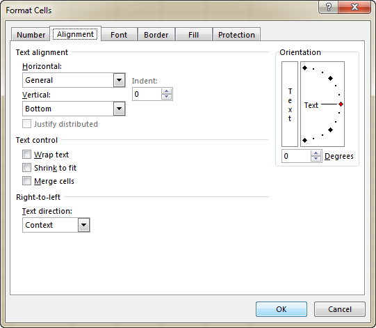
As its name suggests, this tab lets you change text alignment in a cell. Additionally, it provides a number of other options, including:
- Align the cell contents horizontally, vertically, or centered. Also, you can center the value across selection (a great alternative to merging cells!) or indent from any edge of the cell.
- Wrap text into multiple lines depending on the column width and the length of the cell contents.
- Shrink to fit - this option automatically reduces the apparent font size so that all data in a cell fits in the column without wrapping. The real font size applied to a cell is not changed.
- Merge two or more cells into a single cell.
- Change the text direction to define reading order and alignment. The default setting is Context, but you can change it to Right-to-Left or Left-to-Right.
- Change the text orientation. A positive number input in the Degrees box rotates the cell contents from lower left to upper right, and a negative degree performs the rotation from upper left to lower right. This option may not be available if other alignment options are selected for a given cell.
The below screenshot shows the default Alignment tab settings:
Font tab - change font type, color and style
Use the Font tab options to change the font type, color, size, style, font effects and other font elements:

Border tab - create cell borders of different styles
Use the Border tab options to create a border around selected cells in a color and style of your choosing. If you don't want to remove the existing border, select None.
Tip. To hide gridlines in a certain range of cells, you can apply white borders (Outline and Inside) to the selected cells, as shown in the screenshot below:

For more details, see How to create, change and remove Excel cell border.
Fill tab - change the background color of a cell
By using the options of this tab, you can fill cells with different colors, patterns, and special fill effects.

Protection tab - lock and hide cells
Use the Protection options to lock or hide certain cells when protecting the worksheet. For more information, please check out the following tutorials:
Cell formatting options on the ribbon
As you have just seen, the Format Cells dialog provides a great variety of formatting options. For our convenience, the most frequently used features are also available on the ribbon.
Fastest way to apply the default Excel number formats
To quickly apply one of the default Excel formats in terms of number, date, time, currency, percentage, etc., do the following:
- Select a cell or a range of cells whose format you want to change.
- Click the little arrow next to the Number Format box on the Home tab, in the Number group, and select the format you want:

Accounting format options on the ribbon
Apart from changing the cell format, the Number group provides some of the most used Accounting format options:
- To apply Excel Accounting number format with the default currency symbol, select a cell(s), and click the Accounting Number Format icon
 .
. - To choose the currency symbol, click the arrow next to the Accounting Number icon, and select a required currency from the list. If you want to use some other currency symbol, click More Accounting Formats… at the end of the list, this will open the Format Cells dialog with more options.

- To use the thousands separator, click the icon with a comma
 .
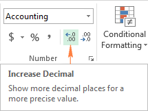
. - To display more or fewer decimal places, click the Increase Decimal or Decrease Decimal icon, respectively. This option can be used for Excel Accounting format as well as for Number, Percentage and Currency formats.
Other formatting options on the ribbon
On the Home tab of the Excel ribbon, you can find far more formatting options such as changing cell borders, fill and font colors, alignment, text orientation, and so on.
For example, to quickly add borders to the selected cells, click the arrow next to the Border button in the Font group, and select the desired layout, color and style:

Excel formatting shortcuts
If you have closely followed the previous parts of this tutorial, you already know most of the Excel formatting shortcuts. The table below provides a summary.
| Shortcut | Format |
| Ctrl+Shift+~ | General format |
| Ctrl+Shift+! | Number format with a thousand separator and two decimal places. |
| Ctrl+Shift+$ | Currency format with 2 decimal places, and negative numbers displayed in parentheses |
| Ctrl+Shift+% | Percentage format with no decimal places |
| Ctrl+Shift+^ | Scientific notation format with two decimal places |
| Ctrl+Shift+# | Date format (dd-mmm-yy) |
| Ctrl+Shift+@ | Time format (hh:mm AM/PM) |
Excel number format not working
If a number of hash symbols (######) appear in a cell after you have applied one of Excel number formats, it's usually because of one of the following reasons:
- The cell is not wide enough to display the data in the selected format. To fix it, all you need to do is increase the column width by dragging the right boundary. Or, double-click the right boundary to automatically resize the column to fit the largest value within the column.
- A cell contains a negative date or a date outside the supported date range (1/1/1900 through 12/31/9999).
To distinguishes between the two cases, hover your mouse over a cell with hash signs. If the cell contains a valid value that is too large to fit in the cell, Excel will display a tooltip with the value. If the cell contains an invalid date, you will be notified about the problem:

This is how you use basic number formatting options in Excel. In the next tutorial, we will discuss the fastest ways to copy and clear cell formatting, and after that explorer advanced techniques to create custom numbers formats. I thank you for reading and hope to see you again next week!
 by
by
47 comments
❤️???
This is very great ?
Hi, I have work sheet in exel example:
1.2
3.5
6.30
9.40
2.50
Now i want to convert or change automatically in exel
A.2
C.E
F.CJ
THAT MEANS I WANT TO USE 1=A, 2=B, 3=C AND .=.
Hi! Use the MID function to extract all the characters from the cell value one by one.
To get the code of the letter corresponding to the digit, add 64 to the digit.
Use the CHAR function to convert code number into alphabet.
Use the ISNUMBER function to convert only numbers to letters.
Use the TEXTJOIN function to combine letters into a text string.
I believe the following formula will help you solve your task:
=TEXTJOIN("",TRUE,IF(ISNUMBER(--MID(A1,ROW(A1:A20),1)), CHAR(MID(A1,ROW(A1:A20),1)+64), MID(A1,ROW(A1:A20),1)))
How can I modify the number of numbers that appear after the decimal point in an Excel file, and make this change permanent and not for specific cells?
Hi! You can change the default number of decimal places in your numbers using Windows Control Panel - Regional Settings: Region and Language > Additional Settings.
hi! I followed the steps and set the default number to 0, but when using Excel, the default number remained 2.
How to convert scientific values to ex: 4.123456781E-05 to 0.0004123456781 in Analysis for Office
Hi! To convert scientific values to decimal number, set the Number format and increase Decimal in the cell. Read more: Custom Excel number format.
When I go to write a figure with a point Double Zero, then double zero could be visible in the Excel cell.
For example,
If I write 745.00, it shows 745 in the Excel Cell.
How can I fix this ?
Hi! If I understand your task correctly, the following tutorial should help: How to control the number of decimal places.
i want to type 5-9 but it is coming in the format 5-may which is not what i want, how can i go About it
Hi!
I recommend add an apostrophe to change number to text format.
I have a number 412345654Q. I want to add spaces such as SSN but it wont since it has a letter at the end. How do I format that column to
show it as 412 345 654Q
Any help would greatly be appreciated!
Hello!
Use the REPLACE function to insert a space at the exact position of the text string.
Try this formula:
=REPLACE(REPLACE(A1,4,0," "),8,0," ")
How do I make a number in hundreds shown in thousands? E.g 645 to convert/show as 645,000. I tried number formatting but the 000 always gets added before 645 -making it to 00645, when I try to customize.
Hi!
If I got you right, try this custom number format:
##",000"
We have a special tutorial on this. Please see: Custom Excel number format
Hi , How I can use TEXT and TODAY function together , I am using =TODAY() for current date and i want to use date in this format 2023-01-25.
but at run time my excel is giving me date like 43221.
Hi!
Set the date format you need in the cell using this instruction: How to change Excel date format and create custom formatting
is there any way to show a blank cell if the cell contains 0 (zero)?
inside the formula, we can use IF to return a blank cell using " "
but I'm looking for constant values in cells
also to show all zero values as a blank cell, we can use FILE>OPTION>ADVANCED>DISPLAY OPTIONS>SHOW A ZERO IN CELLS THAT HAVE ZERO VALUE
but i want not to show zeros in certain cells only,,,,(advanced option doesn't display any zero value)
thanks
Hi!
If I understand correctly, use cell formatting as described in this instruction: Display zeros as dashes or blanks. Hope this is what you need.
your suggestion helped me a lot
thanks
In excel if i ener 356 no. I want this to show in diffrent column like in a 3 in b 5 and in c 7 . Can i do this in excel . And if i put somewher 1,6,9,7,5 then it show me possibilites of no. Like 16975 and 96715
Hi!
I recommend reading this guide: How to split cells in Excel.
Hi i have customer code 11E24 but this is shown as scientific notation how i can solve this
I already format cell
Hi!
Excel shows no more than 15 digits in a number. It shows large numbers in a scientific format. Write your numeric code as text. Try to use the recommendations described in this article: How to convert numbers to text.
I am trying to create a custom format of data.
The number comes in this format :
31026055A but I need it in this format 310-26-055A.
I created a custom format ###-##-### but it doesn't work with the character at the end. What can i use for this?
Hello!
Your value is text, not a number. Therefore, you cannot apply a custom number format. You can change this value in a new cell using text functions.
I'm trying to figure out how to get rid of the dash that Excel puts in place of a 0 in the Accounting format, while retaining the spacing of the $ and the numbers.
Thank you for your help!
Hello!
To turn zeros and dashes into spaces, leave only the currency sign in the third section of the number format. You can add space to align characters in a cell. Read more about it in this guide: Custom Excel number format.
_-* #,##0.00 $_-;-* #,##0.00 $_-;$" ";_-@_-
I hope my advice will help you solve your task.
i am trying to get the average sales per month and my formular isnt updating the rest of the columns. please help.
Hi!
How can I help with the formula if you haven't even written it?
How to write 3-57 in excell, it shows March 57. Pls help
Hello!
If I understand your task correctly, the following formula should work for you:
=TEXT(A1,"mmmm yy")
You can learn more about TEXT function in Excel in this article on our blog.
Hi Premika,
First, set the cell's format to Text, and then type 3-57 in it.
Hi,
Can any one help me to convert scientific notion to the general number for 6.15E+11.
I tried it is giving 615000000000. But this not the right answer.
Hello Manjunath!
So that I can help you, explain what answer you think is right. I would recommend just using a number format.
How do you format a scientific number to a general number? I have occurrences in a spreadsheet and every time I click in the cell I can see the general number on the formula line but in the cell the scientific number still appears.
Hi Leslie,
Just set the Number format for that cell:
1. Select the cell(s), and then open the Format Cells dialog box (Ctrl+1).
2. On the Number tab, select Number under Category.
3. Specify how many decimal places you want to show in a cell and click OK.
-602.11
How do to removed from excel
Hello,
Please specify what exactly you want to remove from Excel.
I'll try to help.
Just a tip regarding the Custom number format - if you have a cell or column that requires a certain number of digits, enter that many zeroes in the "Type" box. If the number is less than that number of digits, it will add leading zeroes to the number. For example, type set to ten zeroes (0000000000) and entry of number 123456 will display as 0000123456.
This also works for long number strings too, where Excel tries to display the number in scientific notation. I often work with 12-digit numbers, and entering 12 zeroes in the type makes Excel display the full number in the cell.
Thank you for this tip, Mikey!
You can find a few more here: Custom Excel number format