The tutorial explains how to use COUNTIFS and COUNTIF formulas with multiple criteria in Excel based on AND as well as OR logic. You will find a number of examples for different data types - numbers, dates, text, wildcard characters, non-blank cells and more.
Of all Excel functions, COUNTIFS and COUNTIF are probably most often mixed up because they look very much alike and both are purposed for counting cells based on the specified criteria.
The difference is that COUNTIF is designed for counting cells with a single condition in one range, whereas COUNTIFS can evaluate different criteria in the same or in different ranges. The aim of this tutorial is to demonstrate different approaches and help you choose the most efficient formula for each particular task.
Excel COUNTIFS function - syntax and usage
The Excel COUNTIFS function counts cells across multiple ranges based on one or several conditions. The function is available in Excel 365, 2021, 2019, 2016, 2013, Excel 2010, and Excel 2007, so you can use the below examples in any Excel version.
COUNTIFS syntax
The syntax of the COUNTIFS function is as follows:
- criteria_range1 (required) - defines the first range to which the first condition (criteria1) shall be applied.
- criteria1 (required) - sets the condition in the form of a number, cell reference, text string, expression or another Excel function. The criteria defines which cells shall be counted and can be expressed as 10, "<=32", A6, "sweets".
- [criteria_range2, criteria2]… (optional) - these are additional ranges and their associated criteria. You can specify up to 127 range/criteria pairs in your formulas.
In fact, you don't have to remember the syntax of the COUNTIF function by heart. Microsoft Excel will display the function's arguments as soon as you start typing; the argument you are entering at the moment is highlighted in bold.

Excel COUNTIFS - things to remember!
- You can use the COUNTIFS function in Excel to count cells in a single range with a single condition as well as in multiple ranges with multiple conditions. If the latter, only those cells that meet all of the specified conditions are counted.
- Each additional range must have the same number of rows and columns as the first range (criteria_range1 argument).
- Both contiguous and non-contiguous ranges are allowed.
- If the criteria is a reference to an empty cell, the COUNTIFS function treats it as a zero value (0).
- You can use the wildcard characters in criteria - asterisk (*) and question mark (?). See this example for full details.
How to use COUNTIFS and COUNTIF with multiple criteria in Excel
Below you will find a number of formula examples that demonstrate how to use the COUNTIFS and COUNTIF functions in Excel to evaluate multiple conditions.
How to count cells with multiple criteria (AND logic)
This scenario is the easiest one, since the COUNTIFS function in Excel is designed to count only those cells for which all of the specified conditions are TRUE. We call it the AND logic, because Excel's AND function works this way.
Formula 1. COUNTIFS formula with multiple criteria
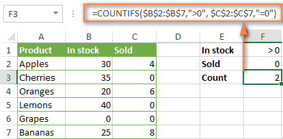
Suppose you have a product list like shown in the screenshot below. You want to get a count of items that are in stock (value in column B is greater than 0) but have not been sold yet (value is column C is equal to 0).
The task can be accomplished by using this formula:
=COUNTIFS(B2:B7,">0", C2:C7,"=0")
And the count is 2 ("Cherries" and "Lemons"):
Formula 2. COUNTIFS formula with two criteria
When you want to count items with identical criteria, you still need to supply each criteria_range / criteria pair individually.
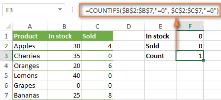
For example, here's the right formula to count items that have 0 both in column B and column C:
=COUNTIFS($B$2:$B$7,"=0", $C$2:$C$7,"=0")
This COUNTIFS formula returns 1 because only "Grapes" have "0" value in both columns.
Using a simpler formula with a single criteria_range like COUNTIFS(B2:C7,"=0") would yield a different result - the total count of cells in the range B2:C7 containing a zero (which is 4 in this example).
How to count cells with multiple criteria (OR logic)
As you have seen in the above examples, counting cells that meet all of the specified criteria is easy because the COUNTIFS function is designed to work this way.
But what if you want to count cells for which at least one of the specified conditions is TRUE, i.e. based on the OR logic? Overall, there are two ways to do this - by adding up several COUNTIF formulas or using a SUM COUNTIFS formula with an array constant.
Formula 1. Add up two or more COUNTIF or COUNITFS formulas
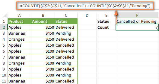
In the table below, supposing you want to count orders with the "Cancelled" and "Pending" status. To have it doen, you can simply write 2 regular Countif formulas and add up the results:
=COUNTIF($C$2:$C$11,"Cancelled") + COUNTIF($C$2:$C$11,"Pending")
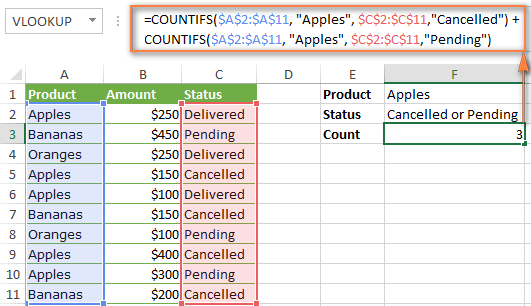
In case each of the functions is supposed to evaluate more than one condition, use COUNTIFS instead of COUNTIF. For example, to get the count of "Cancelled" and "Pending" orders for "Apples" use this formula:
=COUNTIFS($A$2:$A$11, "Apples", $C$2:$C$11,"Cancelled") + COUNTIFS($A$2:$A$11, "Apples", $C$2:$C$11,"Pending")
Formula 2. SUM COUNTIFS with an array constant
In situations when you have to evaluate a lot of criteria, the above approach is not the best way to go because your formula would grow too big in size. To perform the same calculations in a more compact formula, list all of your criteria in an array constant, and supply that array to the criteria argument of the COUNTIFS function. To get the total count, embed COUNTIFS inside the SUM function, like this:
In our sample table, to count orders with the status "Cancelled" or "Pending" or "In transit", the formula would go as follows:
=SUM(COUNTIFS($C$2:$C$11, {"cancelled", "pending", "in transit"}))
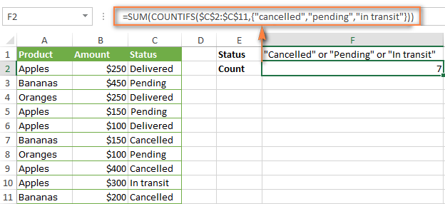
In a similar manner, you can count cells based on two or more criteria_range / criteria pairs. For instance, to get the number of "Apples" orders that are "Cancelled" or "Pending" or "In transit", use this formula:
=SUM(COUNTIFS($A$2:$A$11,"apples",$C$2:$C$11,{"cancelled","pending","in transit"}))

You can find a few more ways to count cells with OR logic in this tutorial: Excel COUNTIF and COUNTIFS with OR conditions.
How to count numbers between 2 specified numbers
By and large, COUNTIFS formulas for numbers fall into 2 categories - based on several conditions (explained in the above examples) and between the two values you specify. The latter can be accomplished in two ways - by using the COUNTIFS function or by subtracting one COUNTIF from another.
Formula 1. COUNTIFS to count cells between two numbers
To find out how many numbers between 5 and 10 (not including 5 and 10) are contained in cells C2 through C10, use this formula:
=COUNTIFS(C2:C10,">5", C2:C10,"<10")
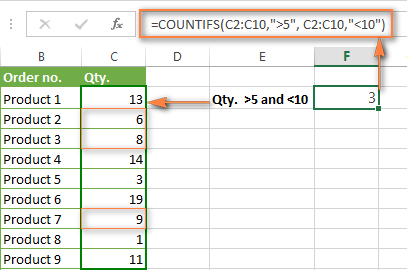
To include 5 and 10 in the count, use the "greater than or equal to" and "less than or equal to" operators:
=COUNTIFS(B2:B10,">=5", B2:B10,"<=10")
Formula 2. COUNTIF formulas to count numbers between X and Y
The same result can be achieved by subtracting one Countif formula from another. The first one counts how many numbers are greater than the lower bound value (5 in this example). The second formula returns the count of numbers that are greater than the upper bound value (10 in this case). The difference between the first and second number is the result you are looking for.
- =COUNTIF(C2:C10,">5")-COUNTIF(C2:C10,">=10") - counts how many numbers greater than 5 and less than 10 are in the range C2:C10. This formula will return the same count as shown in the screenshot above.
- =COUNTIF(C2:C10, ">=5")-COUNTIF(C2:C10, ">10") - the formula counts how many numbers between 5 and 10 are in the range C2:C10, including 5 and 10.
How to use cell references in COUNTIFS formulas
When using logical operators such as ">", "<", "<=" or ">=" together with cell references in your Excel COUNTIFS formulas, remember to enclose the operator in "double quotes" and
add an ampersand (&) before a cell reference to construct a text string.
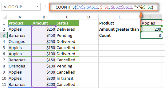
In a sample dataset below, let's count "Apples" orders with amount greater than $200. With criteria_range1 in cells A2:A11 and criteria_range2 in B2:B11, you can use this formula:
=COUNTIFS($A$2:$A$11, "Apples", $B$2:$B$11, ">200")
Or, you can input your criteria values in certain cells, say F1 and F2, and reference those cells in your formula:
=COUNTIFS($A$2:$A$11, $F$1, $B$2:$B$11, ">"&$F$2)
Please notice the use of absolute cell references both in the criteria and criteria_range arguments, which prevents the formula from being broken when copied to other cells.
For more information about the use of an ampersand in COUNTIF and COUNTIFS formulas, please see Excel COUNTIF - frequently asked questions.
How to use COUNTIFS with wildcard characters
In Excel COUNTIFS formulas, you can use the following wildcard characters:
- Question mark (?) - matches any single character, use it to count cells starting and/or ending with certain characters.
- Asterisk (*) - matches any sequence of characters, you use it to count cells containing a specified word or a character(s) as part of the cell's contents.
Tip. If you want to count cells with an actual question mark or asterisk, type a tilde (~) before an asterisk or question mark.
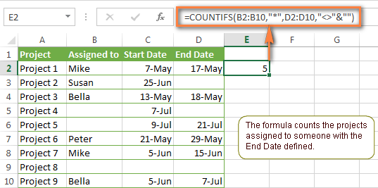
Now let's see how you can use a wildcard char in real-life COUNTIFS formulas in Excel. Suppose, you have a list of projects in column A. You wish to know how many projects are already assigned to someone, i.e. have any name in column B. And because we are learning how to use the COUNTIFS function with multiple criteria, let's add a second condition - the End Date in column D should also be set.
Here is the formula that works a treat:
=COUNTIFS(B2:B10,"*",D2:D10,"<>"&""))
Please note, you cannot use a wildcard character in the 2nd criteria because you have dates rather that text values in column D. That is why, you use the criteria that finds non-blank cells: "<>"&""
COUNTIFS and COUNTIF with multiple criteria for dates
The COUNTIFS and COUNTIF formulas you use for dates are very much similar to the above formulas for numbers.
Example 1. Count dates in a specific date range
To count the dates that fall in a certain date range, you can also use either a COUNTIFS formula with two criteria or a combination of two COUNTIF functions.
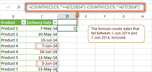
For example, the following formulas count the number of dates in cells C2 through C10 that fall between 1-Jun-2014 and 7-Jun-2014, inclusive:
=COUNTIFS(C2:C9, ">=6/1/2014", C2:C9, "<=6/7/2014")
=COUNTIF(C2:C9, ">=6/1/2014") - COUNTIF(C2:C9, ">6/7/2014")
Example 2. Count dates with multiple conditions
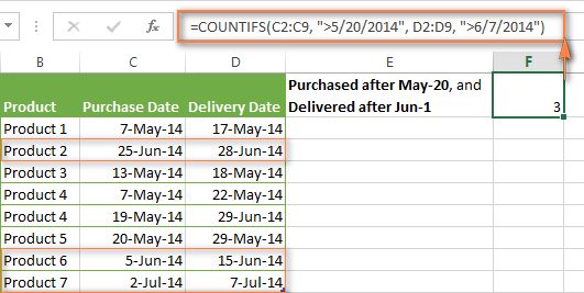
In the same manner, you can use a COUNTIFS formula to count the number of dates in different columns that meet 2 or more conditions. For instance, the below formula will find out how many products were purchased after the 20th of May and delivered after the 1st of June:
=COUNTIFS(C2:C9, ">5/1/2014", D2:D9, ">6/7/2014")
Example 3. Count dates with multiple conditions based on the current date
You can use Excel's TODAY() function in combination with COUNTIF to count dates based on the current date.
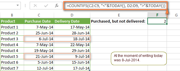
For example, the following COUNTIF formula with two ranges and two criteria will tell you how many products have already been purchased but not delivered yet.
=COUNTIFS(C2:C9, "<"&TODAY(), D2:D9, ">"&TODAY())
This formula allows for many possible variations. For instance, you can tweak it to count how many products were purchased more than a week ago and are not delivered yet:
=COUNTIFS(C2:C9, "<="&TODAY()-7, D2:D9, ">"&TODAY())
This is how you count cells with multiple criteria in Excel. I hope you will find these examples helpful. Anyway, I thank you for reading and hope to see you on our blog next week!
 by
by
1975 comments
Hello
Can you please advise on how to use the COUNTIFS if I would like to calculate occurence of an individual on a rota on weekdays and weekends.
Thank you,
Hello!
To count the number of workdays between two dates, use Excel NETWORKDAYS function. To count weekends, use WORKDAY.INTL function. See the links for examples.
hi,
what is wrong with this syntax ; if the question is ... The choices if "Teacher" or "Student" and under the category "No. Willing to Pay More (PHP 36 - 45 and PHP 46 - 55)"
=COUNTIFS(E5:F19,"Teacher",P5:P19,"ü") note: "ü" character code in excel represents the check mark (✓) character in the column of P5:P19
it will just display an error of "VALUE!
while using...=COUNTIF(E5:F19,"Teacher") and =COUNTIF(P5:P19,"ü") individually has no problem at all..
Thanks so much..Appreciate so much for your immediate response.
Hi!
In the COUNTIFS function, the ranges of values to count must be of the same dimension.
Wonder if you guys could assist... So, i have two columns with unique identifiers, column A = unique identifier 1 and Column B = unique identifier 2... Column A is unique to a record and column B is to distinguish between multiple records so concatenating the two will result in a totally unique value. What i need is a formulae which can count how many lines which are not unique when combined. I'd rather not have another column when concatenated, can this be done in a single formulae?
Hi!
The COUNTIF function can only work with real data ranges. You can't put any other formula in it. Therefore, I cannot help you to count duplicate rows with one formula.
Hello I hope you can help. I've had a read through your tutorial and a few other pages. I'm new to excel but I'm currently building an email tracker for data from Outlook. We use tags on the emails that we can count/filter by. So I can count the amount of times an agents name shows up in total, we also use tags to highlight email types eg New Task, Chase ect. The problem I'm having is that the raw data puts all these tags in the same column in excel separated by a comma.
I have these in a table with agent name in Column A and the email job type in Row 1. If there a way for me to count the amount of times an agent name for example John Smith shows up in the same cell as an email job type for example New Task? The aim is to see how many of each type of email each agent deals with.
When I say "I have these in a table with agent name in Column A and the email job type in Row 1" I mean I am trying to pull the data into a table set out this way.
Hello!
To count data by conditions, split data into separate columns. You can use this guide: Split string by delimiter or pattern, separate text and numbers. To split text into columns by delimiter, you can also use the new TEXTSPLIT function.
Hello, I tried to count all rows containing both, lets say, "Apples" in column A and "Sold" in column B. This works fine, but when I try and count rows containing both, lets say, "Apples" in column A and EITHER "Sold" in column B OR "Sent" in column C, I don't know how to do it. I tried the below, but it double counts if a row fits both the column B and C criteria:
=COUNTIFS(A1:A1000, "Apples", B1:B1000, "Sold") + COUNTIFS(A1:A1000, "Apples", C1:C10, "Sent")
Is there a way to do this without double counting?
Hello!
To count the number of values by OR and AND criteria, use the SUMPRODUCT function. Look for the example formulas here: SUMPRODUCT function with multiple criteria.
=SUMPRODUCT(--(A1:A10="apples"), (B1:B10="sold")+(C1:C10="sent"))
hi im looking for a formula on to automatically count a data if a condition is met....for example
column1(item number) column 2 Column3
1 store1 Pencil
2 store2 Ballpen
3 store2 Paper
4 store1 Eraser
5 Store2 Notebook
6 Store2 paper Clips
7 store1 Calculator
what i want to do is i can automate it into like this
Result1 Store1 Item no. 1, 4, and 7
Result2 Store2 item no. 2-3 and 5 - 6
thanks in advance
Hello!
You can find the examples and detailed instructions here: How to VLOOKUP multiple values in Excel with criteria. I hope my advice will help you solve your task.
big thanks
This is very helpful. I'm trying to use COUNTIFS in a dynamic dropdown list formula with OFFSET and MATCH. Two out of three criteria are a date that falls between two date ranges, but the formula doesn't return the correct values when one date range is non-contiguous. This latter part cannot be helped.
For context:
Columns in ref sheet (TEAMS) are TEAM, MEMBER, JOINDATE, and EXITDATE
The dynamic dropdown formula I'm using is
=OFFSET(Table1[[#HEADERS],[MEMBER]],MATCH(1,([TEAM]=[@TEAM])*([JOINDATE]=[@DATE]),0),0,COUNTIFS([TEAM],[@TEAM],[JOINDATE],"="&[@DATE]))
I have tested this using array and range, and also substituted COUNTIFS with SUMPRODUCT. The result has been the same.
Thanks for your time and help!
Hi, thanks for all the examples. I have a particular one that I haven't been able to figure out.
I need to get a count of particular items that were purchased after a specific date. My example is if I have Apples, Oranges, and pears on a list and I have purchased several of these every day from Sept 1st, 2022 to Oct 31st, 2022. I want to count just pears purchased after Oct 1st, 2022. I have every purchase item listed with it's own date. I just need excel to sort this for me on an excel cell. I can do this through pivot table but this won't help me in this example.
Thank you
Hello!
Use the SUMIFS function to count based on multiple criteria. I recommend reading this guides: Excel SUMIFS date range formula - sum if between two dates and SUMIFS and SUMIF with multiple criteria – formula examples.
I hope I answered your question. If something is still unclear, please feel free to ask.
Hello!
i am trying to calculate & get number of recruiters from a team who has usage >=10 per week
=SUMIFS(DATA[Value],DATA[Folder],"AI",DATA[Delivery Lead],$D44,DATA[Date],Report!E$43,DATA[Value],">="&"10")
I need output as
Name | 10.10.22 | 17.10.22 (Week Start date)
Altaf | 0 | 2 (Two employees has usage >= 10)
Hi!
It is very difficult to understand a formula that contains unique references to your workbook worksheets. Hence, I cannot check its work, sorry.
I'm really Thanks to you and Very useful Information, Examples
hi, how can i make a sum and countifs with mulitple criteria in cell link instead of text? for example: sum(countifs(A3:A7,{"cancelled","apple"})) now instead of using cancelled and apple, i will use cell link like A17 FOR CANCELLED AND A18 FOR APPLE. Is this possible?
Appreciate your help! many thanks
Hello!
If I understand your task correctly, try the following formula:
=SUM(COUNTIFS(A3:A7,A17:A18))
Hi! I hope you can help me I keep getting errors when I try to build this problem into IF and adding multiple => than x.
I am trying to build a formula where I want a blank cell come back with (High, Medium, Low) when there is a specific number in another cell. For instance some types a number between these ranges for High (12 to 13 ), Medium (7 to 11), low (4 to 6)
Hope this makes sense, please advice and your recommendation if any, thank you
Hi!
If I understand your task correctly, you can find the examples and detailed instructions here: Excel nested IF statement - multiple conditions in a single formula.
Hi, thanks a lot for the tips!
Do you know how to count to meet certain criteria continuously instead of just counting overall data?
For e.g.
Inspection result is "PASS" for 60 batches continuously in a specific time range, instead of the normal Inspection results is "PASS" for 60 batches overall in a time range.
Thanks in advance!
Hi!
Have you tried the ways described in this blog post? There are also examples with dates.
I have spent hours trying to make this work. I went through your entire tutorial (which is awesome by the way!) but cannot seem to tweak your formulas to fit my needs where it actually works.
Column M contains dates. I want to find the dates between 9/1/20 and 9/30/20.
Column C contains text. I want to find any matches to the word deviation.
Column E contains text. I want to find all occurrences except cancelled.
I want to count all the instances of occurrences between that date, that match the word deviation, that aren’t cancelled.
I have tried all of these and none work. Can you please help me?
=COUNTIFS(Metrics!M2:M1829,">9/1/2020",Metrics!M2:M1829,"<9/30/2020",Metrics!C2:C1829,"*Deviation*",Metrics!E2:E1829,""&Cancelled)
=COUNTIFS(AND(Metrics!M2:M1829,">9/1/2020",Metrics!M2:M1829,"<9/30/2020"),(Metrics!C2:C1829,"*Deviation*"),(Metrics!E2:E1829,"*Cancelled*"))
=COUNTIFS(Metrics!M2:M1829,">9/1/2020",Metrics!M2:M1829,"<9/30/2020"),(Metrics!C2:C1829,"*Deviation*"),(Metrics!E2:E1829,"*Cancelled*")
=SUM(COUNTIFS(Metrics!M2:M1829,">9/1/2020",Metrics!M2:M1829,"<9/30/2020",Metrics!C2:C1829,"Deviation",Metrics!E2:E1829,"Cancelled")
=SUM(COUNTIFS(Metrics!M2:M1829,">9/1/2020",Metrics!M2:M1829,"<9/30/2020",Metrics!C2:C1829,"Deviation",Metrics!E2:E1829,"Cancelled")
Hello!
If I understand the question correctly, try using the "<>" sign in the condition.
=COUNTIFS(AND(Metrics!M2:M1829,">9/1/2020",Metrics!M2:M1829,"<9/30/2020"), (Metrics!C2:C1829,"<>"&"*Deviation*"), (Metrics!E2:E1829,"<>"&"*Cancelled*"))
Unfortunately that doesn't seem to work. The old "There's a problem with this formula" box comes up. It's highlighted all of the parenthesis, if that's helpful at all.
Hi!
I can't check the formula that contains unique references to your workbook worksheets. Try removing the parentheses from the formula.
=COUNTIFS(Metrics!M2:M1829,">9/1/2020", Metrics!M2:M1829,"<9/30/2020", Metrics!C2:C1829,"<>"&"*Deviation*", Metrics!E2:E1829,"<>"&"*Cancelled*")
Hi,
Am Benson. Can you assist me with a formula to count "number of males, with ages 1 to 4, with a yes on Eligible as seen in the data below
GENDER. AGE. ELIGIBLE
Male 2 Yes
Male 3. Yes
Female 4. Yes
Male. 5. No
Male. 1. Yes
Female. 3. Yes
Male. 2. No
Male. 3. Yes
Female. 5. Yes
Hi!
Please re-check the article above since it covers your case.
Hi,
I'm trying to create a QA scorecard for my team. I hope someone can help me.
What I'm trying to do is that create an point system with my scorecard. Let's say that the passing QA score is 80, that would be equivalent to 30 points. Every time the QA score is deducted with 3, the points will be deducted with 2.
Example:
80 = 30 points
77 = 28 points
73 = 26 points
70 = 24 points
67 = 21 points
and so on.
I'm sorry, there's a mistake. It's supposed to be:
80 = 30 points
77 = 28 points
74 = 26 points
71 = 24 points
68 = 22 points
Hello!
Divide the reduction size by 3 and take the integer part of the number using the INT function. Multiply by 2 and get points.
=INT((80-A1)/3)*2
Note. 67 = 21 points - incorrect.
Im trying to find a formula for the following situation.
I hope I ill be able to explain it clearly.
1 basket contains 3 apples, 4 bananas, 7 oranges
I would like to be able to change the basket number for example to 2 and I would like excel to calculate how many fruits I need for 2 baskets. And when I change it for example to 10 baskets it needs to tell me how many fruits I need to fill each basket.
Thank you for your help
Hello!
If I understand your task correctly, try the following formula:
=A1*3&" apples "&A1*4&" bananas "&A1*10&" oranges"
You can learn more about how to concatenate text strings and another formula in this article: Excel CONCATENATE function to combine strings, cells, columns.
I have a spread sheet that I copy data into from a different spread sheet that tracks quality defects of our products by Date, Model, Serial Number and Production Line. We have some products that have multiple quality issues tied to one serial number that have to be fixed and some that only have one issue.
What I am trying to do is get the count of quality defects by date, but not to include duplicate serial number entries. The formulas below get me different parts of the issues I'm trying to track.
The first one will get me the number of units that had defects that particular day, but it won't exclude the duplicate serial entries.
=COUNTIFS(X2:X1800,"="&DATE(2022,8,22))
The second formula will get me the number of non repeating serial numbers but isn't able to be constrained to a certain date.
=SUM(IF(FREQUENCY(IF(LEN(AE2:AE1800)>0,MATCH(AE2:AE1800,AE2:AE1800,0),""),IF(LEN(AE2:AE1800)>0,MATCH(AE2:AE1800,AE2:AE1800,0),""))>0,1))
So I am needing to figure out a way to combine the formulas so that I can use the same formula in multiple cells but have different dates.
Hello!
You need to use the UNIQUE function to find how many non-repeating serial numbers are for a specific date. The following tutorial should help: How to count unique values with criteria.
I hope it’ll be helpful. If something is still unclear, please feel free to ask.
This Fomula is giving me a Spill error.
=FILTER(A2:A500>="9/1", A2:A500<="9/30")*(COUNTIFS($E$2:$E$500,"*ER*",$I$2:$I$500,"EOU"))
What I am trying to do is in Colum A I have Sept, Oct and Nov dates, which is our Quarter1. Then I have other columns which have drop downs in them (column E and I). So what I need to do is be able to filter these 2 COUNT IFS criteria, by month. And break it out my months within the Quarter 1 spreadsheet tab.
Any assistance would be greatly appreciated!
Hello!
The #SPILL! error occurs when a formula cannot return an array of values to a worksheet. It is possible that the cells already have some values. For more information, please read: Excel #SPILL! error - causes and fixes. I hope I answered your question. If something is still unclear, please feel free to ask.
Hello, I've been struggling with this for some time. I have two sheets.
One sheet has: Sheet two:
COL A|COL B |COL C COL A| COL B| COL C
Player|Week|Points and the other has Name|Name|Both
Objective is to match names in COL A and B from sheet two to COL A in sheet 1.
However the criteria must be-
COL C(Points) must be greater than 26 for the name in COL A( sheet 2)
COL C(Points) must be greater than 20 for the name in COL B(sheet 2)
Both of the above criteria must have been met on the same date.
Any help would be greatly appreciated. the current formula i was trying is:
=COUNTIFS(Table2[FDPoints],">=26",Table2[Player],B75,Table2[Week],10/10/2021)/2+COUNTIFS(Table2[FDPoints],">=20",Table2[Player],F75,Table2[Week],10/10/2021)/2
Hello!
The following tutorial should help: Using Excel COUNTIF function with dates.
I think there is an error in your formula.
Thank you.
So this formula will give me almost what I am looking for:
=COUNTIFS(Table2[Player],[@QB2],Table2[FDPoints],">=26",Table2[Week],"=9/11/2022")+COUNTIFS(Table2[Player],[@RB],Table2[FDPoints],">=20",Table2[Week],"=9/11/2022")
However if one name meets the criteria, it still adds the value. How can I made it add nothing if both names do not match there set criteria.
Example:
1 player has 26 points or over, the other player has 20 points or over. If both are not met, then it does not add.
Currently, if player[QB2] has over 26 points, and player 2[RB] has less than 20, it will return: 1
If both players meet criteria, it returns 2.
I would like for it to be counted as 1 if both criteria is met, but not to count if both are not.
Thank you!
Hi!
If I understand correctly, try to use IF AND function.
=IF(AND(COUNTIFS(Table2[Player],[@QB2], Table2[FDPoints],">=26",Table2[Week],"=9/11/2022")>0, COUNTIFS(Table2[Player],[@RB], Table2[FDPoints],">=20",Table2[Week],"=9/11/2022")>0),1,0)
For more information, please visit: IF AND in Excel: nested formula, multiple statements, and more.
That works perfectly. Now my data contains 18 different dates. Any way to add them up without making a long formula as it will freeze excel if over so many characters?
=IF(AND(COUNTIFS(Table2[Player],[@QB2], Table2[FDPoints],">=26",Table2[Week],"=9/11/2022")>0, COUNTIFS(Table2[Player],[@RB], Table2[FDPoints],">=20",Table2[Week],"=9/11/2022")>0),1,0)+IF(AND(COUNTIFS(Table2[Player],[@QB2], Table2[FDPoints],">=26",Table2[Week],"=1/9/2022")>0, COUNTIFS(Table2[Player],[@RB], Table2[FDPoints],">=20",Table2[Week],"=1/9/2022")>0),1,0)+IF(AND(COUNTIFS(Table2[Player],[@QB2], Table2[FDPoints],">=26",Table2[Week],"=1/2/2022")>0, COUNTIFS(Table2[Player],[@RB], Table2[FDPoints],">=20",Table2[Week],"=1/2/2022")>0),1,0)
etc.
Thanks again
It is actually working great. Thanks for your help!
we have data in column like
AOHO001
AOHO002
AOU1003
AOU2004
AOU3005
AOU1006
AOU2007
AOHO008
we have to count how many no. are AOHO
Hello!
To search for a group of characters in text, use the SEARCH function. Use the ISNUMBER function to determine the cells in which the search was successful.
Please check the formula below, it should work for you:
=SUM(--(ISNUMBER(SEARCH("AOHO",A1:A10))))
plz help me
59 rows 1000 number same then 59 rows 10002 number same then 59 rows 10003 number same in one column .....last 3000 number in excel how to work in excel. plz solve issue.
Hello!
To get a sequence of numbers, use the SEQUENCE function.
You can use this formula:
=CEILING(SEQUENCE(10000,1,1,1)/59,1)+999
Hi there,
Wasn't aware you could use arrays like you've shown. It's much neater.
Is there a way to use an array of Criteria_ranges like this?
The formula I want to use is:
=COUNTIFS(data!$C:$C,Sheet2!$C20,data!N:V,">0.0137",data!N:V,"<0.0432")
I'm aware this doesn't work because of the different size of criteria ranges. Is there any neat / simple way to check each of the columns from N through V for these two conditions, with out writing 18 different range, criteria pairs?
Hope that makes sense. Thanks
Hello!
Try using COUNTIFS for each column, something like this:
=COUNTIFS($C:$C,$C20,N:N,">0.0137",N:N,"<0.0432") + COUNTIFS($C:$C,$C20,O:O,">0.0137",O:O,"<0.0432")+ .........
Read more here: COUNTIF and COUNTIFS with OR conditions.
Please note that if the formula refers to the entire column, then the calculation speed will slow down.
OK. Great thanks.
So there isn't any way to have an array of criteria ranges being checked against a single Criteria?
Hello!
Try SUMPRODUCT function with multiple criteria that can work with arrays.
For example,
=SUMPRODUCT((N:P>0.0137)*(N:P<0.0432)*(A2=$C:$C))
My request is simple for you. I want it to give me a total count if two things in different in to columns (same line) match criteria entered
=COUNTIFS($K$2:$K$5541,"Smith, Mary (56123)",&,$H$2:$H$5541,"BHA")
So if a row contains both Smith, Mary (56123) in one column and BHA is a another column that would be one so 1 would show on the count.
What am I missing?
Hi!
You do not need to use the & operator in the COUNTIFS formula. Try this formula:
=COUNTIFS($K$2:$K$5541,"Smith, Mary (56123)",$H$2:$H$5541,"BHA")
Hi,
Your website is very informative. And I would like to request your help to understand why COUNTIFS function is not working when I add one criterion.
Example data:
Counting Date Material Batch TUID LUID UoM Number of Counts QTY Expected QTY Counted QTY Difference QTY Difference ABS Bin Accuracy
jun 10, 2022 72823224S 21DM14100 104824 1045886 EA 1 2 2 0 0 TRUE
jun 10, 2022 75005333 E75239 125158 1054899 EA 1 16 16 0 0 TRUE
Sheet Raw Data contains (among other columns):
Column A - Counting Date
...
Column L - Bin Accuracy (either True or False)
...
Column O - Is the bin correct? (either Yes or No, and to fill this column I'm using formula =IF(L2="TRUE";"Yes";"No")
Column Q - Business Unit (either O, S or A)
Sheet Results Summary contains (among other columns):
Column DP - Counting Date
Formula =COUNTIFS('Raw Data'!$A:$A,'Results Summary'!DP$1,'Raw Data'!$Q:$Q,"O") is working.
Formula =COUNTIFS('Raw Data'!$A:$A,'Results Summary'!DP$1,'Raw Data'!$Q:$Q,"O",'Raw data'!$L:$L,"FALSE") is not.
I had to use formula =COUNTIFS('Raw Data'!$A:$A,'Results Summary'!DP$1,'Raw Data'!$Q:$Q,"O",'Raw data'!$O:$O,"NO") for it to work.
I thought it could have something to do with the cell format, but I can't seem to find a solution. I already tried changing it to Text, General, but nothing works.
Can you please advise?
Thank you
Hello!
Column L contains boolean values TRUE or FALSE. In your formula, you compare them to the text values "TRUE" or "FALSE". This is not true.
Use
’Raw data’!$L:$L,FALSE and L2=TRUE
Read more about comparing boolean values in this article.
I am using this formula to look in a range and find (match) all instances of the text in "N44", and on the next 7 rows, "N44" becomes "N45", "N46" and so forth, for a list of 8 instances. (i.e., looking for the word "won", "lost", "waiting word".
= COUNTIF('2022'!$K$3:$K$300,N44)
My problem is that I am getting a wrong count. If I personally count in my spreadsheet the instances of "N44", I count one less than what the formula is returning.
The weird part is that not all rows are coming up with the wrong values.
Thank you for your help.
Hi!
I don't have your data, but I'm sure the function is correct. I don't quite understand what "wrong values" means. Perhaps this is the problem.
I have a countifs formula to be able to count the total amount of a selection made in 3 seperate drop down menus. I am not however, able to have the count on all 3 columns of the drop down menus at once (which would be what I need to do).
EX: =COUNTIFS('Juin 2022'!M:M,E2,'Juin 2022'!G:G,C3)
M representing the column of 1 of the drop downs, but I would need N and O also.
Thank you!
Hello!
Have you tried the ways described in this blog post? Pay attention to the following paragraph of the article above - Count cells with multiple criteria (OR logic). If it doesn’t work for you, then please describe your task in detail, I’ll try to suggest a solution.
Hi- Hoping you can help me.
I have two columns of dates: Event Date, and Action Date. There are more Action Dates than Event dates.
These dates are on different worksheets.
I want to find out have many actions happened within 30 days of all of the Event dates
ie, if an event happened on 1/15/22, how many action occurred between 1/15/22 and 2/14/22?
thanks!
Hi!
If you read the last paragraph of this article carefully, you will easily find the answer there.
=COUNTIFS(Sheet1!A1:A10," > ="&DATE(2022,1,15),Sheet1!A1:A10," < ="&(DATE(2022,1,15)+30))
I have a Problem with counting the multiple numbers with "50". Is there a formula to compute how many "50" combining with "today()" formula? Because I want to count all "50" for today only not the whole data set. Hope you can help.
Thank you.
Hi!
I’m sorry but your description doesn’t give me a complete understanding of your task. I'm assuming you want to count the number of values given two conditions. The COUNTIFS function can help you with this. If that's not enough, then explain the issue in more detail.
Hi,
Great tips!
I have a question, do you know how to do the COUNTIFS formula to exclude a word?
So for example, I want two different types of formulas, the first one, I wanna include "word", I did this formula:
=COUNTIFS(Links!J:J,APRIL!E58,Links!M:M,"*word*")
The second one, I want to exclude "word". Is this possible?
Thanks!
Hello!
To exclude “word”, you can subtract its amount from the total number of values.
=COUNTA(Links!M:M) - COUNTIFS(Links!J:J,APRIL!E58,Links!M:M,”*word*”)
I do not recommend using a reference to the entire column in the formula, as this can significantly slow down the calculation.
=SUM(COUNTIF(B2:G2,{"TWG","DEA","FBI","Audit"})*{1,2,3,4})
I am using this formula to assign # values to each text option. So TWG=1, DEA=2, etc. These are trips my company does and the amount of hours each trip is. I am attempting to track how many total hours each colleague has done.
So when I plug in any of those text options in mu table tracking each person's trips, it assigns it a # value and adds up those values in the last column to give me the person's total hours. It works easily, but I don't want to have to keep updating the formula when adding new trip/hour combo (text/# value) .
Is there a way I can put a range of cell values for the criteria and the # values in the above formula? This way I can have a separate table and every time I add a row containing a new trip/hour combo (text/#value) it updates the formula.
Hello!
Write your trips in column A. In columns B and C, write down all the possible travel options and the corresponding number of hours for each of them.
Enter the following formula in cell D1 and then copy it down along the column:
=COUNTIF($A$1:$A$200,B1)*C1
I hope it’ll be helpful.
I'm have a table with as follows:
Item No. --- Sales Order
12345 --- ABCD
54321 --- ABCD
12345 --- EFGH
54321 --- IJKL
What I'm trying to accomplish is COUNTIFS Item No. where Sales Orders Match.
In this case it would be 2, lines 1,2. It's a pretty huge dataset so I was trying to utilize a matrix array of item no x item no and populate. Any thoughts on how this can be accomplished?
Hello!
The answer to your question can be found in this article: Count the total number of duplicates in a column.
This should solve your task.
Hello Team,
Have an interesting problem that we require some help with. We have a daily delivery schedule sheet that comprises of multiple texts with quantity in a single cell. Is there a way to do COUNTIF formula to extract these data? Some of these data do consist of strikethrough data that shouldn't be taken into account.
Also, is there a way to send screenshots so that you will be able to understand the question?
Thank you in advance!
Hi!
Excel formulas cannot determine the format of individual characters in a cell (such as strikethrough characters).
To do mathematical operations with numbers, these numbers must be extracted from text into separate cells.
Please have a look at this articles: How to extract number from string in Excel and
Extract number from string using regular expressions (Regex).
I hope I answered your question. If something is still unclear, please feel free to ask.
Hi all,
Could you please help me to find a formula to count the number of unique values only in one column with a criteria in a another column. Example: There is a column with ID numbers for birds but there are some duplicates (these records must stay in the sheet) and there is a column with a year for when the bird census was done. We need to calculate how many birds with unique id (excluding duplicates) were recorded in Year1, then in Year2 and so on.
Grateful for your assistance.
Hello!
You can find the examples and detailed instructions here: Count unique values with criteria.
=IFERROR(ROWS(UNIQUE(FILTER(A2:A10,B2:B10=E1))), 0)
E1 -- year
I hope this will help.
I have a data set where respondents are allowed to select multiple options (A, B, C, D, E .. etc)
My formula "=countifs($F$2:$F$120, "A", $C$2:$C$120, "Yes")" only shows respondents who only choose "A", but what I want to count are respondents who chose "A" and other options as well.
Would greatly appreciate your help!
Hi!
If all selected options are written in one cell, then you can use the SUMPRODUCT function:
=SUMPRODUCT(--(C1:C120="Yes"), --(ISNUMBER(SEARCH("A",F1:F120))))
If this is not what you wanted, please describe the problem in more detail.
I have a workbook with two tables (A,B). The table I am working in, (A), has descriptions in Column A (Discrepancies found) like:
"1.06. The instrument has been preset"
Table B has headings of Team and several Section x columns. Under each heading is a team name and multiple selections for each Section x for each row. So the Section comment may have more than one entry in each row. I also need to strip the first 6 characters of what is in Column A table A. I use:
=COUNTIFS(Tbl_B[[Team]:[Section 6 Comment]],"*"&MID([@[Discrepancies found]],6,80)&"*") which finds and counts the comment in any of the Section columns for each row of Table fine.
But, I need to count the number of times "The instrument has been preset" occur in each row for those Section columns and Team = "Outgoing". When I try:
=COUNTIFS(Tbl_B[[Team]:[Section 6 Comment]],{"*"&MID([@[Discrepancies found]],6,80)&"*","Outgoing"})
I get an formula error which highlights the second quotation mark from the first asterisk {"*"&MID([@[Discrepancies found]],6,80)&"*" ...}
I have also tried to look across the Sections and Team, but it returns a #Value error:
=COUNTIFS(Tbl_B[[Section 1: Checking Instrument / Customer Settings]:[Section 6 Comment]],"*"&MID([@[Discrepancies found]],6,80)&"*",Tbl_B[Team],"Outgoing")
Figured this out. You can not combine multiple columns with a single column in the Countifs statement. Narrowed to each column and now I can look up multiple items per column. But I loose searching the whole sheet, so I split Table A for each section.
Figured this out. Thanks.
Hi!
It is very difficult to understand a formula that contains unique references to your workbook worksheets. I can't check the formula that contains unique references to your workbook worksheets, sorry.
Give a simpler explanation of your problem. Give an example of the source data and the desired result.
Hi, fisrt I have to say that this posts are SO helpful!
I have a question in the example "Formula 2. SUM COUNTIFS with an array constant" how could I have the count of two different values (apples and oranges) e.g. =SUM(COUNTIFS($A$2:$A$11,"apples","oranges",$C$2:$C$11,{"cancelled","pending","in transit"}))
Thank you!
Hello! I have read through this article a few times and can't figure this out. In my purchases report, say we have the month (ignore the year part) in one column and the item we purchased in another column. Each row is say, a purchase. So I want to know how many keyboards purchased in the month of June. I need a formula that will bring in that information. It will count how many keyboards from one column match up with June in the month column to bring me a count. Can you please assist? I have been working on this one for a while! I have a feeling I have to have multiple commands in the same formula but have come up short.
Thanks!
Hi!
Have you tried the ways described in this blog post? Use the COUNTIFS function with two criteria: month number and product name.
Thanks this has helped keep up the great work.
I was wondering if there was a way to do what I'm trying with one formula instead of multiple?
I am formatting one cell "A1" to indicate if I have any one of the specific items listed more than once in a range.
I have used the below and it does work just wanted to know if there is an easier way with one formula?
The range will have items that are similar like apple or apples2 I'm not interested in those just the ones below and need to know there is more than 1.
formatting rule1
=COUNTIF(range,"apples1")>1
formatting rule2
=COUNTIF(range,"apples3")>1
formatting rule3
=COUNTIF(range,"apples4")>1
List example 1
apples1
apples3
apple
apple
apples4
so nothing of interest is = >1
Do not highlight A1
List example 2
apples1
apples3
apples2
apples2
apples2
apples1
apples4
so
something of interest apples1+apples1= >1
Highlight A1
Hello!
If I understand the problem correctly, you can use an IF function with multiple conditions.
=IF(OR(COUNTIF(range,”apples1″)>1,COUNTIF(range,”apples3″)>1, COUNTIF(range,”apples4”)>1),TRUE,FALSE)
or
=(COUNTIF(range,”apples1″)>1)+(COUNTIF(range,”apples3″)>1)+ (COUNTIF(range,”apples4”)>1)
I hope my advice will help you solve your task.
Hi Team,
Hope you are well.
Kindly advise how to do reverse count? I have data set eg 123,123,123 so when I use countifs, it gives me 3,2,1 but I want 1,2,3 please see the example below. Kindly advise how to solve it?
Number Count I want
123 7 1
123 6 2
123 5 3
123 4 4
123 3 5
123 2 6
123 1 7
124 3 1
124 2 2
124 1 3
125 4 1
125 3 2
125 2 3
125 1 4
COUNTIFS(A2:$A$15,A2)
Thanks
Razib
Hello!
The formula below will do the trick for you:
=COUNTIF($A$2:A2,A2)
After that you can copy this formula down along the column.
Here is the article that may be helpful to you: Relative and absolute cell reference: why use $ in Excel formula
thank you for the Tips what the furmula if I want to says count if The date on Cell A-the date on Cell B> 00 and the cell <0
Hello Team
I have a query regarding CountIfs function for multiple criteria Selection
Here University Name & Session came from a another tab,
When I select the university name as Surrey and Select Session as FA22 so the result will be "2"
Using this Formulla: =sum(COUNTIFS(SFK!$O$8:$O$500,$M$5,SFK!$J$8:$J$500,{$N$4}))
(Sheet Name=SFK , University Name Range=O8:O500 , University Name Selection=M5, Session Range= J8:J500 , Session Selection= N4)
Example
University Name FA22
Surrey 2
Or
When I select the university name as Surrey and Select Session as SP23 so the result will be "1"
University Name SP23
Surrey 1
These two examples are OK for me but the query is " When I select University Name and want all session as a result will be "3" How can I formulate this? I want to Select All Session to get total result also.
Thanks in Advance
Hello!
If I understood you correctly, then the second criterion can be excluded from the formula.
=COUNTIFS(SFK!$O$8:$O$500,$M$5)
We use a monthly schedule to record tasks performed by person. The schedule is a basic grid that has the day of each month in row 1, the task abbreviation in column A and the applicable persons ID is listed in cells B2:AF39.
The second spreadsheet has the full description of each task listed in column A and the person's ID listed in row 1.
I need to count the number of times the ID is listed per task aligning with the ID in cell B1 continuing for all rows/columns.
The formula is in a tab labeled "TasksbyPerson"
=COUNTIFS('MonthlySchedule'!$A:$A,"SMMC 3",'MonthlySchedule'!B:K39,B1)
Hello!
Range B:K39 is not possible. In the COUNTIF and COUNTIFS functions, all ranges must be the same size. These functions cannot solve your problem. Use something like this formula with the SUMPRODUCT function.
=SUMPRODUCT(--((B2:K39="persons ID")*(A2:A39="SMMC 3")))
I hope my advice will help you solve your task.
=COUNTIF(Table3[DATABASE_ROLE],"Primary")-[@[Month Completed]]
What is the purpose of the "@" in this subtraction formula?
Thank you for the tutorial. I have made my school mark sheet through this.
Hello Ablebits team,
I wonder if you could help me. I have a table showing who attended each of our monthly meetings.
I am new to COUNTIF and COUNTIFS and well as fairly new to using tables but would like to use them as the formulas seems to be a little more clearer to read once I get the hang of the syntax. I am not sure if COUNTIF and COUNTIFS can be used in a table
I am counting the number attending and the number of apologies for each meeting. Those I can do with a simple i.e.
Num Present uses "=COUNTIF(Table1[Jun-20],"y")"
Number Apologies (and on leave) uses "=COUNTIF(Table1[Jun-20],"A") +COUNTIF(Table1[Jun-20],"L")"
For the latter I tried to combine the criteria using COUNTIFS i.e.
"=COUNTIFS(Table1[Jun-20],"=A", Table1[Jun-20],"=L")" but that didn't work.
My main problem is that I want to count the number of people eligible to attend any particular meeting.
The reason for that is that over time some people may have been employed after the date for that month's record or may have left their job before that meeting.
I tried to do this by comparing a start date and end date with the date of the meeting. I had a problem because I was using the meeting date as a column heading and realised that I can't compare date values to a column heading text. I overcame that by putting the month date in a separate row above the table headings.
I would appreciate it if you could provide some guidance on how to create functional formula to do this.
My table structure is as follows (which you can paste into a text file and open it as CSV.
The table is between rows 5 and 14, with row 5 as the heading.
Attendance at monthly meetings,,Total Available,0,
,,Present,3,
,,Apologies/Leave,2,
Put Date in this row and label in the one below so we can use it in formulas,,,12-May-20,
Person,Start Month,End Month,May-20,
Person 1,21-Jan-18,,y,
Person 2,21-Mar-18,29-Jul-19,,
Person 3,1-Feb-20,,y,
Person 4,1-Mar-18,,L,
Person 5,1-Apr-21,1-Jun-20,,
Person 6,1-Feb-20,1-Jun-20,A,
Person 7,1-Mar-20,,y,
Person 8,1-Jul-20,,,
Person 9,6-Jul-20,,,
Hello!
To convert a date as text to a normal date, use the DATEVALUE function.
I hope I answered your question. If something is still unclear, please feel free to ask.
I want to count a column of criteria where V=1 and v=.5 and the total would be the # of Vs and v's combined, but can't figure out how to make the formula have v=.5 instead of 1, as the countifs function counts the numberof cells not the value of the cell data.
Is there a function that will essentially add up all the V's and v's in a column for a combined total ( eg: there are 4 Vs and 2vs for a total of 5. I want to basically do a sum where V=1 and v=.5
Hello!
Multiply the number of found values 0.5 by 0.5 and get their sum. I hope I understood the problem correctly.
Greetings: my organization uses a scheduling calendar that can export information to Excel such that calendar dates are populated along the x-axis and individual names are on the Y-axis. Each cell will be assigned a text value that represents the shift assignment for the day for the individual designated on the Y-axis.
I’m trying to create a count of days for an entire year, for each individual, which correlates the assignment designated “A” with any number of assignments, call them “B,C,D,E” that occurs the calendar day immediately BEFORE assignment “A”. Only one assignment for the preceding day “B, C, D OR E) would need to be found to increase the count. How could I write an appropriate formula which would count the cells where assignment (B,C,D OR E) is followed by assignment “A” ? Would it be easier if the data was transposed such that the individual populate the X axis and dates the Y axis?
Thank you for your assistance.
Hello!
If the data for a person is recorded in the range B2:N2, then the count of the cells according to your conditions can be calculated using the formula
=SUM(((TRANSPOSE(B2:N2)="B")+ (TRANSPOSE(B2:N2)="С")+ (TRANSPOSE(B2:N2)="D")+ (TRANSPOSE(B2:N2)="E"))* (TRANSPOSE(C2:O2)="A"))
I hope my advice will help you solve your task.
I want to count the number of specific values in a column (F:F) that fall between two dates (the start and finish of the month) contained in another column (H:H).
The values in F:F are one of 29 specificvalues and column H:H contains dates from 01/01/22-
31/12/22(updated daily)
I want to be able to count how many of the specific values F:F appear in any given month.
I can count each specific value F;F with the formula =COUNTIF('2022'!F:F,"*51/1 assault*")
I can count the total number of values F:F appearing between two dates with the formula =COUNTIFS('2022'!H:H,">="&DATE(2022,2,1),'2022'!H:H,"<="&DATE(2022,2,28))
But I just can't work out how to count a particular value in any given month.
Can you help me?
Hi!
Try to merge formulas:
=COUNTIFS(‘2022′!H:H,”>=”&DATE(2022,2,1),’2022’!H:H,”<="&DATE(2022,2,28),‘2022’!F:F,”*51/1 assault*”)
Kindly I need your help
My manager asked me about the excel sheet if we can fix .
the vacant bed which highlighted in green color in the excel sheet it is the result of difference of night shift census (J25) minus Total bed capacity bed(C25) minus total blocked bed (T25) . however he need if the night shift not filled the result will be day shift census minus Total bed capacity bed(C25) minus total blocked bed (T25) . If both them filled will be calculated only the night shift census (J25) minus Total bed capacity bed(C25) minus total blocked bed (T25) .
How we can do that in excel sheet
Hoping for your help in this matter .
Thank you very much
Best Regards
Hello!
Unfortunately, I could not understand your conditions for counting. Could you please describe it in more detail? Give an example of the source data and the expected result.
Hi!
Your description doesn’t give me a complete understanding of your task. You did not provide the addresses of all the cells, but the formula could be something like this:
=IF(J25<>"",J25-C25-T25,A25-C25-T25)
I recommend that you carefully study the article - How to use IF function in Excel