Microsoft Excel provides several functions purposed for counting different kinds of cells, such as blanks or non-blanks, with number, date or text values, containing specific words or character, etc.
In this article, we will focus on the Excel COUNTIF function that is purposed for counting cells with the condition you specify. First, we will briefly cover the syntax and general usage, and then I provide a number of examples and warn about possible quirks when using this function with multiple criteria and specific types of cells.
In essence, COUNTIF formulas are identical in all Excel versions, so you can use the examples from this tutorial in Excel 365, 2021, 2019, 2016, 2013, 2010 and 2007.
COUNTIF function in Excel - syntax and usage
Excel COUNTIF function is used for counting cells within a specified range that meet a certain criterion, or condition.
For example, you can write a COUNTIF formula to find out how many cells in your worksheet contain a number greater than or less than the number you specify. Another typical use of COUNTIF in Excel is for counting cells with a specific word or starting with a particular letter(s).
The syntax of the COUNTIF function is very simple:
As you see, there are only 2 arguments, both of which are required:
- range - defines one or several cells to count. You put the range in a formula like you usually do in Excel, e.g. A1:A20.
- criteria - defines the condition that tells the function which cells to count. It can be a number, text string, cell reference or expression. For instance, you can use the criteria like these: "10", A2, ">=10", "some text".
And here is the simplest example of Excel COUNTIF function. What you see in the image below is the list of the best tennis players for the last 14 years. The formula =COUNTIF(C2:C15,"Roger Federer") counts how many times Roger Federer's name is on the list:
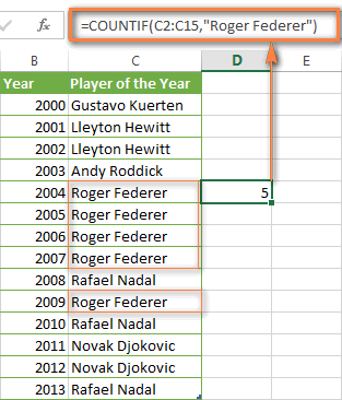
Note. A criterion is case insensitive, meaning that if you type "roger federer" as the criteria in the above formula, this will produce the same result.
Excel COUNTIF function examples
As you have just seen, the syntax of the COUNTIF function is very simple. However, it allows for many possible variations of the criteria, including wildcard characters, the values of other cells, and even other Excel functions. This diversity makes the COUNTIF function really powerful and fit for many tasks, as you will see in the examples that follow.
COUNTIF formula for text and numbers (exact match)
In fact, we discussed the COUNTIF function that counts text values matching a specified criterion exactly a moment ago. Let me remind you that formula for cells containing an exact string of text: =COUNTIF(C2:C15,"Roger Federer"). So, you enter:
- A range as the first parameter;
- A comma as the delimiter;
- A word or several words enclosed in quotes as the criteria.
Instead of typing text, you can use a reference to any cell containing that word or words and get absolutely the same results, e.g. =COUNTIF(C1:C9,C7).
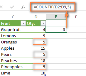
Similarly, COUNTIF formulas work for numbers. As shown in the screenshot below, the below formula perfectly counts cells with quantity 5 in Column D:
=COUNTIF(D2:D9, 5)
In this article, you will find a few more formulas to count cells that contain any text, specific characters or only filtered cells.
COUNTIF formulas with wildcard characters (partial match)
In case your Excel data include several variations of the keyword(s) you want to count, then you can use a wildcard character to count all the cells containing a certain word, phrase or letters as part of the cell's contents.
Suppose, you have a list of tasks assigned to different persons, and you want to know the number of tasks assigned to Danny Brown. Because Danny's name is written in several different ways, we enter "*Brown*" as the search criteria =COUNTIF(D2:D10, "*Brown*").
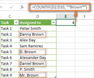
An asterisk (*) is used to find cells with any sequence of leading and trailing characters, as illustrated in the above example. If you need to match any single character, enter a question mark (?) instead, as demonstrated below.
Tip. It is also possible to use wildcards with cell references with the help of the concatenation operator (&). For example, instead of supplying "*Brown*" directly in the formula, you can type it in some cell, say F1, and use the following formula to count cells containing "Brown": =COUNTIF(D2:D10, "*"&F1&"*")
Count cells beginning or ending with certain characters
You can use either wildcard character, asterisk (*) or question mark (?), with the criterion depending on which exactly result you want to achieve.
If you want to know the number of cells that start or end with certain text no matter how many other characters a cell contains, use these formulas:
=COUNTIF(C2:C10,"Mr*") - count cells that begin with "Mr".
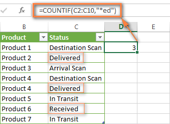
=COUNTIF(C2:C10,"*ed") - count cells that end with the letters "ed".
The image below demonstrates the second formula in action:
If you are looking for a count of cells that start or end with certain letters and contain the exact number of characters, you use the Excel COUNTIF function with the question mark character (?) in the criteria:
=COUNTIF(D2:D9,"??own") - counts the number of cells ending with the letters "own" and having exactly 5 characters in cells D2 through D9, including spaces.
=COUNTIF(D2:D9,"Mr??????") - counts the number of cells starting with the letters "Mr" and having exactly 8 characters in cells D2 through D9, including spaces.
Tip. To find the number of cells containing an actual question mark or asterisk, type a tilde (~) before the ? or * character in the formula. For example, =COUNTIF(D2:D9,"*~?*") will count all cells containing the question mark in the range D2:D9.
Excel COUNTIF for blank and non-blank cells
These formula examples demonstrate how you can use the COUNTIF function in Excel to count the number of empty or non-empty cells in a specified range.
COUNTIF not blank
In some Excel COUNTIF tutorials and other online resources, you may come across formulas for counting non-blank cells in Excel similar to this one:
=COUNTIF(A1:A10,"*")
But the fact is, the above formula counts only cells containing any text values including empty strings, meaning that cells with dates and numbers will be treated as blank cells and not included in the count!
If you need a universal COUNTIF formula for counting all non-blank cells in a specified range, here you go:
Or
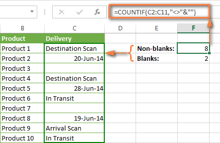
This formula works correctly with all value types - text, dates and numbers - as you can see in the screenshot below.
COUNTIF blank
If you want the opposite, i.e. count blank cells in a certain range, you should adhere to the same approach - use a formula with a wildcard character for text values and with the "" criteria to count all empty cells.
Formula to count cells not containing any text:
Since an asterisk (*) matches any sequence of text characters, the formula counts cells not equal to *, i.e. not containing any text in the specified range.
Universal COUNTIF formula for blanks (all value types):
The above formula correctly handles numbers, dates and text values. For example, here's how you can get the number of empty cells in the range C2:C11:
=COUNTIF(C2:C11,"")
Please be aware that Microsoft Excel has another function for counting blank cells, COUNTBLANK. For instance, the following formulas will produce exactly the same results as the COUNTIF formulas you see in the screenshot above:
Count blanks:
=COUNTBLANK(C2:C11)
Count non-blanks:
=ROWS(C2:C11)*COLUMNS(C2:C11)-COUNTBLANK(C2:C11)
Also, please keep in mind that both COUNTIF and COUNTBLANK count cells with empty strings that only look blank. If you do not want to treat such cells as blanks, use "=" for criteria. For example:
=COUNTIF(C2:C11,"=")
For more information about counting blanks and not blanks in Excel, please see:
COUNTIF greater than, less than or equal to
To count cells with values greater than, less than or equal to the number you specify, you simply add a corresponding operator to the criteria, as shown in the table below.
Please pay attention that in COUNTIF formulas, an operator with a number are always enclosed in quotes.
| Criteria | Formula Example | Description |
|---|---|---|
| Count if greater than | =COUNTIF(A2:A10,">5") | Count cells where value is greater than 5. |
| Count if less than | =COUNTIF(A2:A10,"<5") | Count cells with values less than 5. |
| Count if equal to | =COUNTIF(A2:A10,"=5") | Count cells where value is equal to 5. |
| Count if not equal to | =COUNTIF(A2:A10,"<>5") | Count cells where value is not equal to 5. |
| Count if greater than or equal to | =COUNTIF(C2:C8,">=5") | Count cells where value is greater than or equal to 5. |
| Count if less than or equal to | =COUNTIF(C2:C8,"<=5") | Count cells where value is less than or equal to 5. |
You can also use all of the above formulas to count cells based on another cell value, you will just need to replace the number in the criteria with a cell reference.
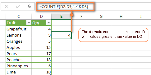
Note. In case of a cell reference, you have to enclose the operator in quotes and add an ampersand (&) before the cell reference. For example, to count cells in the range D2:D9 with values greater than a value in cell D3, you use this formula =COUNTIF(D2:D9,">"&D3):
If you want to count cells that contain an actual operator as part of the cell's contents, i.e. the characters ">", "<" or "=", then use a wildcard character with the operator in the criteria. Such criteria will be treated as a text string rather than a numeric expression. For example, the formula =COUNTIF(D2:D9,"*>5*") will count all cells in the range D2:D9 with contents like this "Delivery >5 days" or ">5 available".
Using Excel COUNTIF function with dates
If you want to count cells with dates that are greater than, less than or equal to the date you specify or date in another cell, you proceed in the already familiar way using formulas similar to the ones we discussed a moment ago. All of the above formulas work for dates as well as for numbers. Let me give you just a few examples:
| Criteria | Formula Example | Description |
|---|---|---|
| Count dates equal to the specified date. | =COUNTIF(B2:B10,"6/1/2014") | Counts the number of cells in the range B2:B10 with the date 1-Jun-2014. |
| Count dates greater than or equal to another date. | =COUNTIF(B2:B10,">=6/1/2014") | Count the number of cells in the range B2:B10 with a date greater than or equal to 6/1/2014. |
| Count dates greater than or equal to a date in another cell, minus x days. | =COUNTIF(B2:B10,">="&B2-"7") | Count the number of cells in the range B2:B10 with a date greater than or equal to the date in B2 minus 7 days. |
Apart from these common usages, you can utilize the COUNTIF function in conjunction with specific Excel Date and Time functions such as TODAY() to count cells based on the current date.
| Criteria | Formula Example |
|---|---|
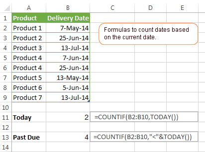
| Count dates equal to the current date. | =COUNTIF(A2:A10,TODAY()) |
| Count dates prior to the current date, i.e. less than today. | =COUNTIF(A2:A10,"<"&TODAY()) |
| Count dates after the current date, i.e. greater than today. | =COUNTIF(A2:A10,">"&TODAY()) |
| Count dates that are due in a week. | =COUNTIF(A2:A10,"="&TODAY()+7) |
| Count dates in a specific date range. | =COUNTIF(B2:B10, ">=6/1/2014")-COUNTIF(B2:B10, ">6/7/2014") |
Here is an example of using such formulas on real data (at the moment of writing today was 25-Jun-2014):
Excel COUNTIF with multiple criteria
In fact, Excel COUNTIF function is not exactly designed to count cells with multiple criteria. In most cases, you'd use its plural counterpart, the COUNTIFS function to count cells that match two or more criteria (AND logic). However, some tasks can be solved by combining two or more COUNTIF functions in one formula.
Count values between two numbers
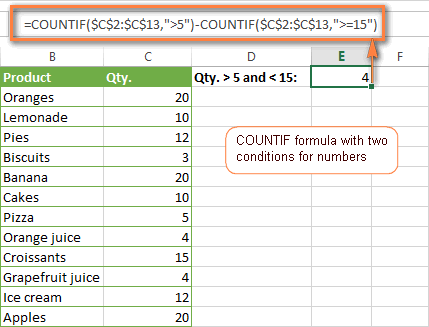
One of the most common applications of Excel COUNTIF function with 2 criteria is counting numbers within a specific range, i.e. less than X but greater than Y. For example, you can use the following formula to count cells in the range B2:B9 where a value is greater than 5 and less than 15.
=COUNTIF(B2:B9,">5")-COUNTIF(B2:B9,">=15")
How this formula works:
Here, we use two separate COUNTIF functions - the first one finds out how many values are greater than 5 and the other one gets a count of values greater than or equal to 15. Then, you subtract the latter from the former and get the desired result.
Count cells with multiple OR criteria
In situations when you want to get several different items in a range, add 2 or more COUNTIF functions together. Supposing, you have a shopping list and you want to find out how many soft drinks are included. To have it done, use a formula similar to this:
=COUNTIF(B2:B13,"Lemonade")+COUNTIF(B2:B13,"*juice")
Please pay attention that we've included the wildcard character (*) in the second criterion, it is used to count all kinds of juice on the list.
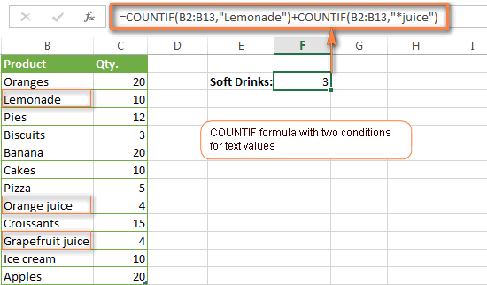
In the same manner, you can write a COUNTIF formula with several conditions. Here is an example of the COUNTIF formula with multiple OR conditions that counts lemonade, juice and ice cream:
=COUNTIF(B2:B13,"Lemonade") + COUNTIF(B2:B13,"*juice") + COUNTIF(B2:B13,"Ice cream")
For other ways to count cells with OR logic, please see this tutorial: Excel COUNTIF and COUNTIFS with OR conditions.
Using COUNTIF function to find duplicates and unique values
Another possible usage of the COUNTIF function in Excel is for finding duplicates in one column, between two columns, or in a row.
Example 1. Find and count duplicates in 1 column
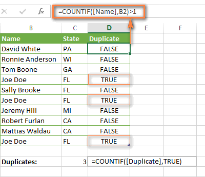
For example, this simple formula =COUNTIF(B2:B10,B2)>1 will spot all duplicate entries in the range B2:B10 while another function =COUNTIF(B2:B10,TRUE) will tell you how many dupes are there:
Example 2. Count duplicates between two columns
If you have two separate lists, say lists of names in columns B and C, and you want to know how many names appear in both columns, you can use Excel COUNTIF in combination with the SUMPRODUCT function to count duplicates:
=SUMPRODUCT((COUNTIF(B2:B1000,C2:C1000)>0)*(C2:C1000<>""))
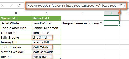
We can even take a step further and count how many unique names there are in Column C, i.e. names that do NOT appear in Column B:
=SUMPRODUCT((COUNTIF(B2:B1000,C2:C1000)=0)*(C2:C1000<>""))
Tip. If you want to highlight duplicate cells or entire rows containing duplicate entries, you can create conditional formatting rules based on the COUNTIF formulas, as demonstrated in this tutorial - Excel conditional formatting formulas to highlight duplicates.
Example 3. Count duplicates and unique values in a row
If you want to count duplicates or unique values in a certain row rather than a column, use one of the below formulas. These formulas might be helpful, say, to analyze the lottery draw history.
Count duplicates in a row:
=SUMPRODUCT((COUNTIF(A2:I2,A2:I2)>1)*(A2:I2<>""))
Count unique values in a row:
=SUMPRODUCT((COUNTIF(A2:I2,A2:I2)=1)*(A2:I2<>""))

Excel COUNTIF - frequently asked questions and issues
I hope these examples have helped you to get a feel for the Excel COUNTIF function. If you've tried any of the above formulas on your data and were not able to get them to work or are having a problem with the formula you created, please look through the following 5 most common issues. There is a good chance that you will find the answer or a helpful tip there.
1. COUNTIF on a non-contiguous range of cells
Question: How can I use COUNTIF in Excel on a non-contiguous range or a selection of cells?
Answer: Excel COUNTIF does not work on non-adjacent ranges, nor does its syntax allow specifying several individual cells as the first parameter. Instead, you can use a combination of several COUNTIF functions:
Wrong: =COUNTIF(A2,B3,C4,">0")
Right: =COUNTIF(A2,">0") + COUNTIF(B3,">0") + COUNTIF(C4,">0")
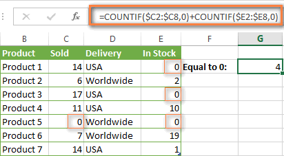
An alternative way is using the INDIRECT function to create an array of ranges. For example, both of the below formulas produce the same result you see in the screenshot:
=SUM(COUNTIF(INDIRECT({"B2:B8","D2:C8"}),"=0"))
=COUNTIF($B2:$B8,0) + COUNTIF($C2:$C8,0)
2. Ampersand and quotes in COUNTIF formulas
Question: When do I need to use an ampersand in a COUNTIF formula?
Answer: It is probably the trickiest part of the COUNTIF function, which I personally find very confusing. Though if you give it some thought, you'll see the reasoning behind it - an ampersand and quotes are needed to construct a text string for the argument. So, you can adhere to these rules:
If you use a number or a cell reference in the exact match criteria, you need neither ampersand nor quotes. For example:
=COUNTIF(A1:A10,10)
or
=COUNTIF(A1:A10,C1)
If your criteria includes text, wildcard character or logical operator with a number, enclose it in quotes. For example:
=COUNTIF(A2:A10,"lemons")
or
=COUNTIF(A2:A10,"*") or =COUNTIF(A2:A10,">5")
In case your criteria is an expression with a cell reference or another Excel function, you have to use the quotes ("") to start a text string and ampersand (&) to concatenate and finish the string off. For example:
=COUNTIF(A2:A10,">"&D2)
or
=COUNTIF(A2:A10,"<="&TODAY())
If you are in doubt whether an ampersand is needed or not, try out both ways. In most cases an ampersand works just fine, e.g. both of the below formulas work equally well.
=COUNTIF(C2:C8,"<=5")
and
=COUNTIF(C2:C8,"<="&5)
3. COUNTIF for formatted (color coded) cells
Question: How do I count cells by fill or font color rather than by values?
Answer: Regrettably, the syntax of the Excel COUNTIF function does not allow using formats as the condition. The only possible way to count or sum cells based on their color is using a macro, or more precisely an Excel User-Defined function. You can find the code working for cells colored manually as well as for conditionally formatted cells in this article - How to count and sum Excel cells by fill and font color.
4. #NAME? error in the COUNTIF formula
Issue: My COUNTIF formula throws a #NAME? error. How can I get it fixed?
Answer: Most likely, you have supplied an incorrect range to the formula. Please check out point 1 above.
5. Excel COUNTIF formula not working
Issue: My COUNTIF formula is not working! What have I done wrong?
Answer: If you have written a formula which is seemingly correct but it does not work or produces a wrong result, start by checking the most obvious things such as a range, conditions, cell references, use of ampersand and quotes.
Be very careful with using spaces in a COUNTIF formula. When creating one of the formulas for this article I was on the verge of pulling my hair out because the correct formula (I knew with certainty it was right!) wouldn't work. As it turned out, the problem was in a measly space somewhere in between, argh... For instance, look at this formula:
=COUNTIF(B2:B13," Lemonade").
At first sight, there is nothing wrong about it, except for an extra space after the opening quotation mark. Microsoft Excel will swallow the formula just fine without an error message, warning or any other indication, assuming you really want to count cells containing the word 'Lemonade' and a leading space.
If you use the COUNTIF function with multiple criteria, split the formula into several pieces and verify each function individually.
And this is all for today. In the next article, we will explore several ways to count cells in Excel with multiple conditions. Hope to see you next week and thanks for reading!
 by
by
1059 comments
I am trying to do a monthly resource prediction so want to keep the month start /end date- either as a formula or cell reference. My formula is not throwing any error but not showing the result
While this one works
=COUNTIFS(F1:F116,"OFFSHORE",Roster!$I$1:$I$116,"BAU",I1:116, "INFRA",H1:H116,">=01-sep-2023")
when i put the date 01-sep-2023 as a cell and refer to that in the formula
=COUNTIFS(F1:F116,"OFFSHORE",Roster!$I$1:$I$116,"BAU",I1:116, "INFRA",H1:H116,">="&B1)
while it is not throwing any error but it is not fetching either
Hi! You may have the date written as text in cell B1. Try using this instruction: How to insert date in Excel.
I am trying to get a count of cells based off of multiple conditions including a date reference from a different cell. I had a conditional format changing the cells colors based on the date but couldn't get a count from the conditional format. After trying a few VBA's that I found no luck. I then thought maybe I could combine my conditional format formula with my COUNTIF formula but it's still not working. My formulas are =COUNTIF(C6:AG6, "A")+COUNTIF(C6:AG6, "NCNS") and for the conditional one its =C5<=TODAY()-180. Is there a way I can get a count using the two formulas together? Any help is greatly appreciated. Thank you
If you want to calculate values only if the condition with cell C5 is TRUE, you can combine the two formulas into one using multiplication:
=(COUNTIF(C6:AG6, "A")+COUNTIF(C6:AG6, "NCNS")) * (--(C5<=TODAY()-180))
Hi, I have a long column with dates of the form: month/day/year. How can I count the number of times one particular year shows up in the column?
Hi,
I would like to ask if there's a formula that meet the following criteria.
a. Unique Order ID will be counted by day (e.g. Mon-Fri) in a week (e.g. weeknum 1-52) from yesterday's date after 10 am until before 10 am the next day
b. and the Orders created from Fri after 10 am, Sat and Sun will be added to Mon orders before 10 am
Really appreciate your help.
Thank you.
Order ID Order Date Order Time WeekDay WeekNum
A 1-Jan-23 3:45:11 Sun 1
B 1-Jan-23 3:45:08 Sun 1
C 1-Jan-23 20:45:11 Sun 1
D 1-Jan-23 3:45:11 Sun 1
E 1-Jan-23 3:45:10 Sun 1
F 1-Jan-23 18:46:15 Sun 1
O 2-Jan-23 18:45:32 Mon 1
P 2-Jan-23 8:45:12 Mon 1
Q 2-Jan-23 13:45:42 Mon 1
R 2-Jan-23 9:46:39 Mon 1
S 2-Jan-23 2:45:23 Mon 1
T 2-Jan-23 10:45:58 Mon 1
how many orders drop every day based on the criteria
WeekNum Mon Tue Wed Thu Fri
1
2
3
4
5
6
7
8
Hi! If I understood the question correctly, add 10 hours to the date written in D1 using the TIME function and count the cells matching the conditions using the SUMPRODUCT function.
=SUMPRODUCT((A1:A20>=(D1+TIME(10,0,0)))*((A1:A20<=(D1+1+TIME(10,0,0)))*B1:B20))
25.06.2023 aa
26.06.2023 bb
27.06.2023
28.06.2023 cc
29.06.2023
30.06.2023
01.07.2023 dd
02.07.2023
I want to count, how many in June and July ? The answer is June = 3 and July = 1
Hi! All the conditions you are talking about are described in the article above. Apply them in the COUNTIFS function.
=COUNTIFS(A2:A10,">=1.6.2023",A2:A10,"<=30.6.2023",B2:B10,"<>")
Thank you very much.
Nama buah|jumlah
-----------------------------
apel | 5
anggur | 3
apel | 4
nah saya mau mencari jumlah apel di kolom a2-a4. namun di kalikan dulu apet tadi dengan angka di kolom b2-b4.
perhitungan manualnya begini.
(a2*ba)+(a4*b4)
nah. begitu rumusnya giman ya?
Makasih sebelumnya.
Please re-check the article above since it covers your case.
I want to count a range of numbers, however, some of the number have a + in front of the integer and some don't. For example, +2.5 and +7. In order to get the "+" I used the apostrophe. EG: '+3. Can I now count a range of any numbers between +3 and +7? I assume that using the apostrophe turns it to text and there is no way to still count without asking Excel to COUNTIF '+1 and COUNTIF '+2, etc., etc.?
Thanks.
Hi! Using an apostrophe turns numbers into text. You can get + in before positive numbers by using a custom number format: +##;-##.
Hi,
I need help with a formula, i am wanting to count columns that have a value greater than 0 but only if the date is a weekday, The colums are labeled by date only.
I am currently using this formula which counts any cell including weekend days.
=COUNTIF(D2:AL2,">0")
Hi! To determine the day of the week, use the WEEKDAY function. The formula below counts days except Saturday and Sunday.
=SUM(--(WEEKDAY(D2:G10,2)<6))
I have spent many hours on here. I want to count how many, say appointments a person has in a given month. I'm not even to going to try to factor in asking to also include initials of people, that's clearly too much to ask. Trying the following:
=COUNTIF(O2:O2974, ">=01/07/2023")-COUNTIF(O2:O2974, "<31/07/2023") As in the range from 01/07/2023 to the end of that month. Getting a 'zero'. Any help much appreciated thanks.
Hi! Use ">31/07/2023" in your formula. Pay attention to the following paragraph of the article above: Using Excel COUNTIF function with dates.
Hi,
I'm strugling with very simple formula:
=countif($a$1:a1,a1)
I just want to count and to number in a2 all unique and duplicate values.
Formula works perfect for static column (a1), but once I start to insert new data in column a1 - I get an error.
Thank you in advance.
Hi! I don't really understand what you want to do. A1 is a cell, not a column. Explain how you want to number unique values and duplicates. Look carefully at the examples above. I kindly ask you to take a closer look at the following paragraph of the article above: Count duplicates and unique values.
Hi,
I have One item duplicated in two rows, second item duplicated item in three rows, third item duplicated in four rows. Total three different items in 9 rows; how can I get the total number of each specific duplicated items using excel formula?. The answer should be 3 (Apple, Orange, Lemon).
e.g.
Apple
Apple
Orange
Orange
Orange
Lemon
Lemon
Lemon
Lemon
Hi! The following tutorial should help: Excel UNIQUE function - fastest way to find unique values.
I am trying to create a formula where excel looks for a specific name (down column A) on a separate page in the workbook & then looks across when it finds the name to count how many times they picked that week. I can’t get any formula to work I figured Countifs would do the trick. However, I keep getting an error.
I tried for example =countifs(!’Sunday Schedule’A2:A20, “John Doe”, !’Sunday Schedule’B2:P25, “PICK”).
Hi! The cell ranges you use in a COUNTIF or COUNTIFS formula must be the same size. For example,
=countifs(A2:A20, “John Doe”, B2:P20, “PICK”)
Also pay attention to how to make a reference to another sheet or workbook (external reference).
Sir Want to count amount against the specific date (mention in column a) while amount is enter in column b, can you help me?
Example : Column a containing on date (1-30 each Month)
Column b containing on amount received in different sights, know i want to count whole amount which received on the same date,
Hi! You can find the examples and detailed instructions here: Excel SUMIFS date range formula - sum if between two dates.I hope it’ll be helpful.
I'm trying to get a count of items that were completed after their due date. So in the below, Column G shows the due date, and then when the item is completed we enter the completion date into Column I. So I was trying to do a formula that would just compare if the date in Column G is less than its counterpart in Column I. Is there any way to do this without creating a new column with a =IF($G1<$I1,"Paste Due","On Time") and then counting that column?
Column G Column I
Due Date Completed Date
1/1/23 1/1/23
1/10/23 1/15/23
1/31/23
2/5/23 2/3/23
I tried
=COUNTIF(G:G<I:I)
but that gives me a "#SPILL!" error in my formula cell.
Hi!
The formula below will do the trick for you:
=SUM(--(G1:G100<I1:I100))
Double minus converts TRUE and FALSE to 1 and 0.
I want to make a count per day for a type of task. this would be a running total throughout a week Sunday through Saturday.
If i select PLP in Cell D and it occurs on a Sunday which is in Cell C, then i want a running count on my summary sheet to show 1 for Sunday, Since this task is done up to 8 times daily I want to know how many throughout the day per day for the week. Appreciate any incite.
I got it finally, it would let me delete, Thank you
=COUNTIFS('Audit Tracker'!D$2:D$300, "PLP", 'Audit Tracker'!C$2:C$300, "Sunday")
I am trying to develop a statement which will count the number of cells in Col A which meet ALL 3 of the following criteria:
- the Year in the cell in Col A must = Today's Year
- the Month in the cell in Col A must = Today's Month
- the Day in the cell in Col A must >= Today's Day
The data beginning in Col A1 is as follows (all of the dates are in date-defined cells and there may be some cells with text (such as "Date" in A1 or left blank such as in A6):
Date
05/10/23
06/15/23
09/15/23
12/15/24
07/15/23
10/15/23
01/15/23
05/15/23
The formula I created is:
=COUNT(IF(AND(YEAR(A:A)=YEAR(TODAY()),MONTH(A:A)=MONTH(TODAY())),DAY(A:A)>=DAY(TODAY())),1)
The result is 1 even though the dates in cells A2 (05/10/23) and A10 (05/15/23) both meet all 3 conditions and should therefore return a result of 2.
Please help to understand where I have gone wrong. Thanks!
Hi! I don't really understand why A10 (05/15/23) meets today's day.
Hi, I thought that A10 would qualify as its day (the 15th) is greater than or equal to today's day.
PS - As a further test, I changed all of the dates to be non-qualifying (none of the years = 2023, none of the months = 5 and none of the days are >= today's day), but the result remains 1. I also deleted all of the dates, but the result continues to be 1. I must not understand correctly how the IF/Count statement works. Thanks.
Hi!
If I understand your task correctly, the following formula should work for you:
=COUNTIF(A2:A10,">="&TODAY())
For more information, please read: Using Excel COUNTIF function with dates.
Thanks so much
This is more of a COUNT issue than a COUNTIF but not sure if COUNTIF is what I need. I have the following formula
=COUNT(IF(MONTH('Iveco-Home'!$M:$M)=12,1)), which looks for the month December. However I am trying to move it on a month to January but blank cells are reporting as January too, how do I get my formula to avoid the blanks? Thank you in advance
Hi! To exclude empty cells, add an AND condition to the IF formula.
Please try the following formula:
=COUNT(IF(AND(MONTH('Iveco-Home'!$M:$M)=1, 'Iveco-Home'!$M:$M >0),1))
Something isn't working and I can't see what the issue is. The data below is for column M:M but the formula is returning a value of 0 when I am expecting 1.
Current del date
Oct-23
Oct-23
Oct-23
Oct-23
Jan-24
Any help greatly appreciated.
I placed your data in column M. The formula works.
Sorry to revisit this again but I am still struggling to get the formula to work. I created a new document just with the following data
Oct-23
Oct-23
Oct-23
Oct-23
Jan-24
and I could get the formula to work, however if I had more Jan dates I am still getting a result of 1?
Again any help greatly appreciated.
Hi! Try another version of the formula to count all the January dates and ignore the blank cells.
=SUM((MONTH(M1:M100)=1)*(M1:M100>0))
Hi,
I want to pick "out" & "in" from a specific data rows, Which formula will work in excel without using text to column. As I have thousands of rows.
Admitted 'Harold Nelson, John' (Card: 817252) at 'METRO-PRODUCTION WALDO RECEPTION' (OUT) entering area METRO AREA INTERNAL.
Admitted 'Harold Nelson, John' (Card: 817252) at 'METRO-PRODUCTION WALDO RECEPTION' (IN) entering area METRO AREA PRODUCTION WALDO.
Admitted 'Rojas Salas, Jorgue' (Card: 817218) at 'METRO-PRODUCTION WALDO RECEPTION' (IN) entering area METRO AREA PRODUCTION WALDO.
Admitted 'ESPINOSA, CARLOS ANDRES' (Card: 622867) at 'METRO-PRODUCTION WALDO RECEPTION' (IN) entering area METRO AREA PRODUCTION WALDO.
Admitted 'Harold Nelson, John' (Card: 817252) at 'METRO-PRODUCTION WALDO RECEPTION' (IN) entering area METRO AREA PRODUCTION WALDO.
Hi! Your task is not completely clear to me. To understand what you want to do, give an example of the desired result.
Hi
I am searching to find/count the intermediate holidays between two holidays or the current day depending on the date & day. In the following table Dates 3 and 10 are weekend Fridays. I want to count employee's Present (P), Absent (A) or Leave (SL/CL) depending on attendance, i.e. if an employee is present on the day before and after the weekend then the day off is counted as present. and if he is absent or on leave on the days before and after the weekend, his weekend will be counted as absent or holiday.
Name Designation 01 02 03 04 05 06 07 08 09 10 11 12 13 14 15 16 P SL CL EL SPL LWP A - WHD
Mr. A Abc P P P P P P P P P P P P P P 14 - - - - - - - 2
Mr. B Def P P P P A P P p P P P P P P 13 - - - - - - 1 2
Mr. C Ghi P P P P LWP P P A A SPL P P P P 10 - - - 1 1 2 2
Mr. D Jkl P P P P P P P CL CL P SPL P P P 11 - 2 - 1 - 1 - 2
Thank you.
I'm trying to count cells with TRUE or FALSE in them.
The TRUE or FALSEs were gotten out of an IF function.
But anytime I use COUNTIF([cell range]),"TRUE"), I am getting 0.
Why is it so, and what is the right thing to do?
Thank you.
Hello!
The IF function returns a boolean TRUE or FALSE value, not a text value. Do not use quotes in your formula.
COUNTIF([cell range]),TRUE)
unfortunately, I tried the formula without the quotes, but I still get 0 as output. COUNTIF([cell range]),TRUE)
Hi!
Read carefully in the article above how to use the COUNTIF formula. For example,
=COUNTIF(B2:B10,TRUE)
the problem is the closed bracket after the [cell range]
From your post COUNTIF([cell range]),TRUE)
need to change to COUNTIF([cell range],TRUE)
COUNTIF([cell range],TRUE)
so it's looking for blanks.
I'm trying to figure out a countif formula for Days Open based off today.
90 Days Open
Working off the below list.
4/10/2022 4:00 1
4/10/2022 4:01 11
4/17/2022 4:01 4
4/21/2022 12:35 2
4/21/2022 12:39 1
4/24/2022 4:00 5
4/24/2022 4:00 1
5/29/2022 4:00 10
Any idea how to do this?
Hi!
I kindly ask you to have a closer look at the following paragraph of the article above: COUNTIF formulas for dates
Hi,
What formula can i use if i want to count a specific timeframe?
Ex.
Column A
1:15 AM
1:30 AM
2:15 AM
2:30 AM
in Column B i want an output that will indicate how many are in range of 1AM-1:59AM
in column C i want an output that will indicate how many are in range of 2AM-2:59AM
Thanks
Hi!
Pay attention to the following paragraph of the article above – Excel COUNTIF with multiple criteria.
It covers your case completely.
Or you can use the COUNTIFS function: How to count numbers between 2 specified numbers.
Hello!
I am in a pickle and could use some help.
With what kind of formula can I count years?
I have a list:
1 year; 0 months
2 years; 2 months
1 year; 0 months
0 years; 4 months
3 years; 3 months
1 year; 0 months
And so on.
I would like to count them like this
<1 year; 0 months
1 year; 0 months <2 years 0 months
And so on
Hello!
Split years and months into two columns. See recommendations: Split string by delimiter or pattern, separate text and numbers.
Extract the numbers from the text of these two columns to use the COUNTIFS function. For more information, please visit: Extract number from text string.
I Want to count if the value is =>6 count 6,if Value is 7-15 count 10, if value is 16-30 count 15, if value is 30-90 count 20 and if value is 90-200 count 50, and if value is 200 > count 100
DOH Count
15 10
23 15
0 6
107 50
50 20
239 100
5 6
would you please help to solve this issue?
Hi!
See the second paragraph of this article for an example of a solution to your problem: Excel nested IF statement - multiple conditions in a single formula.
How to count only Dates in a column withh dates and names
Hi!
Dates are numbers. Therefore, to count dates, you can use the COUNT function. It ignores text.
Hi,
I've been looking through the blogs about COUNTIFS, VLOOKUP, IF and DATES, but it still puzzles me. I'm in need of the formula to seek for the latest date (Column A) on a specific items (Column B) for its amount (Column C) to show up in a new column. For instance, I would required the latest amount of Item A on 5/3/22, which is supposed to come back at 6. Anything after 5/3/22 should not reflect in the new column.
Column A
2/3/22
4/3/22
5/3/22
5/3/22
6/3/22
6/3/22
6/3/22
Column B
Item A
Item B
Item A
Item A
Item A
Item A
Item B
Column C
4
4
5
6
5
3
5
Hello!
Use the XMATCH function to search from last to first.
=INDEX(C1:C7,XMATCH(1,($A$1:$A$7=F1)*($B$1:$B$7=G1),0,-1))
I hope my advice will help you solve your task.
Hi,
I've tried on the formula given but it does not come back with any number. Instead, it only shows "#NAME?" in the column.
Hi,
I've gone through some checking and found out that the XMATCH function only applicable to Excel 365 above. I'm currently using an Excel 2019 which did not support the new function. Would hope that there is a formula to reflect the previous formula given in Excel 2019.
Thank you
Hello!
To find the last match in a range of data, select the row with the highest row number using the MAX function. Use this array formula:
=INDEX($C$1:$C$7, MAX(($A$1:$A$7=F1)*($B$1:$B$7=G1)*ROW($A$1:$A$7)))
Press Ctrl + Shift + Enter so that array function works.
Hi Alex,
Thank you for the wonderful formula. The formula works perfectly fine, but only if the first row starts with Row 1. If I were to start it on other rows, the formula will not come back to the designated results be it array function or not. For instance, if I started it out with Row 2, an array function will come back with 5 and without the array function will come back with 4. What was the issue that caused for the differences?
Hello!
Subtract from the row number the number of rows before the start row. If it starts on line 2, then subtract 1.
=INDEX($C$2:$C$8,MAX(($A$2:$A$8=F1)*($B$2:$B$8=G1)*(ROW($A$2:$A$8)-1)))
Hi Alex,
Fantastic! Thank you once again for your assistance. Very much appreciated.
How to use COUNTIF to count the number of times a cell appears in a range.
For Example: in cells C10:C33 I have equations, and I want to know within that cell range how many times F2 appears in the equation.
This is to track an expenditure “automatically”
If COUNTIF cannot be used for this then what is your suggestion?
Hello!
If I understand the problem correctly, get the text of the formula using the FORMULATEXT function and find the text "F2" using the SEARCH function.
=COUNT(SEARCH("F2",IFERROR(FORMULATEXT(C2:C20),"")))
Hope this is what you need.
Thanks for your reply, interestingly it doesn’t want to acknowledge that we’re doing a range. I tested it on single cells and it works, giving me a value of 1 when it contains “F2” and 0 when it doesn’t.
Once I introduce the range of C10:C33 it just gives me a value of 1 instead of counting the entire range.
It’s a problem with the formulatext only accepting the first cell in the range.
Hi!
If you have Excel 2019 and earlier, try writing this formula as an array formula using Ctrl + Shift + Enter, not just Enter. For more information, please visit: Excel array formula examples for beginners and advanced users.
I am going crazy and am new to spreadsheets.
I am using
=COUNTIF($D$53:$D$82,"Yes")/COUNTIF($D$53:$D$82,"*")
This range is 31 cells and represents days in the month. The result is reading as [0/32 days] - which is very close to what I need except the range should read /31 days. I'm boggled.
Hi!
This range is 30 cells.
I tried using the countifs formula to know the number of items within a specfic date range..
Apple jan-april total 100
It worked well.
But when I tried to use the same formula in finding the total number of apples per month. It doesnt seem right.
Because when i tried to add the number of apples from jan - apr, im not getting the total 100 from the 1st formula.
Can someone pls help?
Hi!
I don't know what formula you are using and can't see your data. Please re-check the article above since it covers your task. Or describe the problem in more detail.
Is there a way to count only the cells in a row that have visible data? Meaning it doesn't count cells with formulas in it when the formula is telling the cell not to show anything, like by using "" ?
Thanks for your consideration.
Hello!
If I understood correctly, check the value "" in the cell. For example,
=COUNTIFS(A1:A5,"<>",A1:A5,"="&"")
Thanks for your very useful blog.
I just wish to know how you display the results of countifs. for example if I wish to find numbers >= 5 in a long list of numbers, countif return their count but I need to display also the numbers or list of numbers which is/are greater or equal to 5.
Best Wishes
Ali
Hello!
To display a list of values by condition, use the FILTER function.
The formula might look like this:
=FILTER(C2:C20,C2:C20>=5,"")
Thanks a lot.
But filter function didn't work in excel 2016 any other suggestions?
Hi. How do I get a count for years of service when my cells have decimals (must keep the decimals)? Example: If I have services ranging between 0-55 years and I want to calculate how many have worked for 5 years, but I have some at 5.1, others at 5.4, 5.7, etc. How do I calculate how many of employees are celebrating their 5 years (including 5 to up to 5.9, but not 6) this fiscal year?
I tried these: =COUNTIF(J2:J113,">=5*=5=5"); =COUNTIF(J2:J113,"*~5*"); =COUNTIF(J2:J113,"~5*"); =COUNTIF(J2:J113,"~5.*"); =COUNTIF(J2:J113,"*5.*"); =COUNTIF(J2:J113,"5.?"); =COUNTIF(J2:J113,"5."); =COUNTIF(J2:J113,"5"); =COUNTIF(J2:J113,"=5""=5""=5,<=6"), and countless others, but they don't work.
What am I missing? I just want to know how many people to celebrate in increments of 5s at our facility, but can adjust the formula once I have the 5 years ones.
Thank you in advance for your help.
Blessings.
Oh my goodness! Could it be =COUNTIF(J2:J113,">=4.5")-COUNTIF(J2:J113,">6") ?!
As soon as I posted my frustrated question, I thought of this one. Is this correct?
Hello!
To count the number of values in an interval, use the COUNTIFS function with two conditions:
=COUNTIFS(J2:J113,">="&5,J2:J113,"<"&10)
Or use two COUNTIF functions:
=COUNTIF(J2:J113,">="&5)-COUNTIF(J2:J113,">"&10)
Hello,
This Formula works =COUNTIFS(COUNT, B26, CO, "FSC",STATUS, "OVERDUE") but I want to a count of how many OVERDUE are over 120 Days.
B26 = the Category
CO = the B Column
STATUS = the F Column and OVERDUE is in that Column
DAYS = Column G
I want a count of the category specified that is in the CO specified that has a status of OVERDUE with days that are greater than or equal to 120.
Any Ideas?
Hi!
Read the article above carefully, it contains the answer to your questions.
I don't know how the days are written in column G. If it's a number, then the condition is ">="&120
If it is a date, then the condition is "<="&(TODAY()-120)
For more information about counting with multiple conditions using the COUNTIFS function, see this article.
Hello,
Thank you for your reply! It is a number and I want to count how many with that name have a number greater than higher than 120 in column G. and I have read this multiple times and I cant get it to do what i want. I'm not that smart, which is why I asked all of you (The Smart Ones) the question. I tried =COUNTIFS(COUNT, B27, CO, "FSC",STATUS, "OVERDUE",">="&120) and it says "You've entered too few arguments for this function". I have a cell that counts if the name in B27 that has a company "FSC" that has a Status of "OVERDUE" and it works but I need to know how many of those with that name, company, and status are equal to or over the number (120) in a different column.
Thank you
Just to be clear I I have tried more that one string. I have tried multiple in different variations to include dates with =COUNTIFS(COUNT, B27, CO, "FSC",STATUS, "OVERDUE","<="&TODAY()-120) and everything in the article that made since to what I was trying to accomplish ( In my option, I very well could be wrong and answer is staring me right in the face ( I've staring at this spreadsheet for a couple weeks now)).
Hi!
Try the following formula:
=COUNTIFS(COUNT, B27, CO, "FSC",STATUS, "OVERDUE",G:G,">="&120)
Thank you for you response!
I tried it with no luck, it says #VALUE! where the count should be. I tried this a couple of different ways with the same out come.
Hi, I am looking to compare first and last names from two different sheets. First sheet is our master registration with over 500 names on it. Second sheet (and subsequent sheets) is/are individual event(s) that someone is signed up for.
Column A is last name
Column B is first name
Column C on "Master Registration" sheet is the first event
Column D on "Master Registration" sheet is the second event....and so forth
I would like to have Columns C, D, etc. return a value to indicate the different events that someone is signed up for, based upon second, third, fourth sheets.
The issue I am having: first and last names are separated into separate columns...
Any help would be greatly appreciated. Thank you very much.
Hello!
If the second sheet (and subsequent sheets) also has columns with first name and last name, then try using the guide: Excel INDEX MATCH with multiple criteria.
I hope it’ll be helpful. If something is still unclear, please feel free to ask.
how this if(countif(A$1:A1,A1)=1 formula works
Where (A$1:A1) & (A$1:A1,A1) is used
Hi!
Your formula is incorrect and cannot work
I am trying to set up a vacation tracker where every V for vacation is counted as 1 and every .5V is counted as a half day. I tried to do a countif, but couldn't get it to work.
Hi!
Count with COUNTIF first with V, then with the second formula with 0.5V. Multiply the second result by 0.5 and sum both results.
Hi Alexander!
This may sound really silly, but here's the question: I have one row of numbers where I am adding all numbers in the row
1 2 3 4 5 6 7 8 9 10 11 12 etc
How do i get the count of cells until the sum in the row is less than or equal to 21?
The answer of count must be of course 6
Hello!
On a separate row, calculate the running total.
Then, use the MATCH function to find the first value in that row that is greater than 21.
=MATCH(TRUE,A2:Z2>21,0)-1
Thank you Alexander!
Just in time for handing the excel which is due today!
Have a good one
Hi there,
Lets say I have this situation
A B C D E
A1 B1 C1 D1 E1
A+ B+ C+ D+ E+
A- B- C- D- E-
I would like to get all values of letter A
please help.
Hi!
The following tutorial should help to get a list of unique values with the letter A: Get a list of unique values based on criteria.
Here's an example of a formula:
=UNIQUE(FILTER(A1:A10,ISNUMBER(SEARCH("A",A1:A10))))
Hello! Sorry, why in the formula for calculating COUNTIF within a range
=COUNTIF(B2:B9,">5")-COUNTIF(B2:B9,">=15") there's a greater-than sign before 15? Shouldn't it be a less-than sign (<)? Thanks
Hello!
Unfortunately, you are mistaken. The formula counts values greater than 5 and then subtracts the number of values greater than 15. As a result, we get the number of values greater than 5 but less than 15.
Will countif function counts cells with formulas in it?
Hi!
Of course. The COUNTIF function counts values that are written manually or obtained using formulas.
Hi! I have been working on a formula and I wanted to ask if there is a workaround it. Columns C-O has data validation in it (Yes/No). For Column P (Remarks) wanted to do a sanity check so I have this formula =IF(COUNTIF(C1:O1,"No")>0,"Incomplete","Complete"). The default remark is complete - I wanted to know if the default remark can be blank instead of complete? Thank you.
Hello!
If I understood correctly, you can use an empty string in the IF function instead of a text value.
=IF(COUNTIF(C1:O1,"No")>0,"Incomplete","")
Hi,
Please help with this task.
I want to list the names who have not participated but registered for the period of last week (which starts on Monday) by comparing the list of participants.
Column A: contains participants
Column B: contains the date
Column C: registered members
Thank you
Hello!
Please check out the following article on our blog, it’ll be sure to help you with your task: Compare two columns for matches and differences.
I hope my advice will help you solve your task.
I am trying to figure how to count an item
ex. I have a set of dates throughout the year in 1 column and I have another column with a word in it; ex. open or closed.
I am trying to see how I can count either open or closed from the date column?
Hello!
Please check out this article to learn how to calculate values by condition.
I hope this will help.
what is the difference between =COUNTIF('sheetName'!B2:B15, "=PASS") and =COUNTIF(sheetName!B2:B15, "=PASS")?
thank you
branko
Hi Branko,
If the sheet name includes spaces or non-alphabetical characters, it must be enclosed in single quotation marks. If the sheet name includes only letters, numbers and underscores, single quotes are not needed. For example, to refer to "Sheet1", you'd use the reference Sheet1!B2:B15. To refer to "Sheet 1", the reference is 'Sheet 1'!B2:B15.
For more information, please see How to refer to another sheet or workbook in Excel.
I have a large excel file with a lot of data.
I know how to delete the duplicate values but keep one value.
I need to learn another technique.
For example, a particular column repeats some data twice, some data thrice, and some data for four or five times.
I want to delete the first entry only. I don't want to delete the second, third or fourth entry. That means only the first entry or first data will be deleted, but all the second, third, fourth or the next entry will exist.
Will you please tell me how I can do this?
Hello!
To determine the 1st occurrence of the duplicate, write down the formula in the additional column:
=IF(AND(COUNTIF($A$2:$A$9, A3)>1,COUNTIF($A$2:$A3, A3)=1), "1st occurrence", "")
In this case, your list begins at cell A3. Copy the formula down the column as needed.
Hi, Can u help me
ive got several problems with my excel worksheet>
im trying to figure out how to count some data with random data like this :
Dates 02/01/22 03/01/22 04/01/22 05/01/22 06/01/22 07/01/22 08/01/22
Name
Yoga CT PL CT CT PL DL DL
and i want to get (CT) count data with range number that i provide from another cell, so ijust need to fill my range date cell and get total data number :
A1 A2 A3
Data Range 02/01/2022 04/01/22
Thank u so much
appreciate
Hi!
If I understood correctly, you have several conditions for counting values. Use the COUNTIFS function for this.
I hope it’ll be helpful.
The tutorial Excel COUNTIF for blank and non-blank cells contains numerous errors.
COUNTIF(range,"*")
The tutorial states that this formula counts only cells containing any text values. It does not mention that it also will not count cells containing null text values that are the result of a formula.
Consider a cell containing the formula =IF(D52908="kMDItemUserTags = (",MID(D52909,5,99),""). Note that the result of this can be, in fact usually is, null, i.e. zero in length. When the condition is false, the result of the COUNTIF function is wrong.
This can be tested by having a cell with the formula ="" in the range of the COUNTIF function.
COUNTIF(range,"")
and
COUNTIF(range,""&"")
These also fail when a cell within the range contains a null value that is a result of a function.
In the screenshot show in the tutorial, placing the formula ="" in cells C4 and C8 will illustrate this.
COUNTIF(range,""&"*")
Again, This also fails when a cell within the range contains a null value that is a result of a function.
COUNTIF(range,"")
Finally, a formula that works when the range contains formulas generating null values.
But why use the COUNTIF function at all? Just using the COUNTBLANK(range) function will be simpler and more descriptive.
But, all these (COUNTIF and COUNTBLANK) functions also fail if the range contains cell which contain one, or more, spaces, whether keyed in or the result of a formula. In other words, the length of the cell is greater than zero but the data consists only of spaces. Excel, apparently, does not consider spaces to be blank.
Hello Mark,
Thank you for your feedback. I will try to clarify the two main points.
Zero-length strings. In terms of Excel, an empty string ("") is a text value - ISTEXT returns TRUE for it. The COUNTA function also regards zero-length strings as non-empty cells. Given the above, it's incorrect to say that COUNTIF formulas fail in this scenario as their results are consistent with the results of other Excel functions.
Spaces. Like zero-length strings, spaces (and other non-printable characters) are text values. Therefore, cells containing only spaces are not considered empty and are not counted by COUNTBLANK or analogous COUNTIF formulas.
Why do we use the COUNTIF function for counting blank/non-blanks? At the very least, to show that Excel provides different ways to accomplish the same task :) Of course, there is also a practical application - knowing how to express such criteria, you can build more sophisticated COUNTIFS formulas, say, to count rows that have blanks in one column and non-blanks in another.
Hi,
I am trying to create a dynamic formula for the below table to count no of invoices(unique).. When I use countif function the output which I am getting is counting all the row's. For Eg Doc # 20212463 this will be counted as 2 instead of 1
I am looking for a formula like this - in the month of Sep on Thursday at 12 .00pm how many unique invoices were created. I really appreciate if you can help me with this.
Doc # Wk day Time Month
20212463 Tue 16:00 Aug-21
20213081 Thu 19:00 Oct-21
20212463 Tue 16:00 Aug-21
20212704 Thu 12:00 Sep-21
20212960 Wed12:00 Oct-21
20212704 Thu 12:00 Sep-21
20212705 Thu 12:00 Sep-21
20212706 Thu 12:00 Sep-21
20212707 Thu 12:00 Sep-21
20212708 Thu 12:00 Sep-21
20212488 Fri 17:00 Sep-21
20212702 Wed 16:00 Sep-21
20213074 Wed 14:00 Oct-21
20212489 Fri 18:00 Sep-21
20212292 Fri 22:00 Aug-21
20212382 Sat 20:00 Aug-21
20212788 Thu 18:00 Sep-21
20213086 Fri 17:00 Oct-21
20212292 Fri 22:00 Aug-21
20212292 Fri 22:00 Aug-21
20212292 Fri 22:00 Aug-21
20212292 Fri 22:00 Aug-21
20212292 Fri 22:00 Aug-21
Hello!
To count unique values by condition, you can find the examples and detailed instructions here: How to count unique values in Excel with criteria.
This should solve your task.
Sir
can you please send this excel file on email
COUNTIF in Excel - count if not blank, greater than, duplicate or unique
Hi,
Pls suggest me a formula if i want to count total particular time (hr:min) from given range of time.
i.e. if somebody have performed shift duty from evening 20:00 o’clock to morning 8:00 o’clock and i want to count hours from 22:00hrs to 6:00hrs for that particular shift !
So what formula will come there ?
Thanks.
Hi!
If the end time is longer than the start time, then you need to add 1 day to their difference
=IF(A1 > A2,A2-A1+1,A2-A1)
Hi, please could you help. I am trying to count: I have a document of customer sales on my store,
column A is style codes/skus (which will be duplicated). column b is units sold,
I want to count the units in column B when they match a specific style code in column A so that I can see how many in total sold of a specific style.
I have read this doc thoroughly and cannot seem to find a way to work it.
many thanks!
Hello!
I think in order to calculate the amount of sales of a product, you need to use the SUMIF function.