The tutorial explains how to use COUNTIFS and COUNTIF formulas with multiple criteria in Excel based on AND as well as OR logic. You will find a number of examples for different data types - numbers, dates, text, wildcard characters, non-blank cells and more.
Of all Excel functions, COUNTIFS and COUNTIF are probably most often mixed up because they look very much alike and both are purposed for counting cells based on the specified criteria.
The difference is that COUNTIF is designed for counting cells with a single condition in one range, whereas COUNTIFS can evaluate different criteria in the same or in different ranges. The aim of this tutorial is to demonstrate different approaches and help you choose the most efficient formula for each particular task.
Excel COUNTIFS function - syntax and usage
The Excel COUNTIFS function counts cells across multiple ranges based on one or several conditions. The function is available in Excel 365, 2021, 2019, 2016, 2013, Excel 2010, and Excel 2007, so you can use the below examples in any Excel version.
COUNTIFS syntax
The syntax of the COUNTIFS function is as follows:
- criteria_range1 (required) - defines the first range to which the first condition (criteria1) shall be applied.
- criteria1 (required) - sets the condition in the form of a number, cell reference, text string, expression or another Excel function. The criteria defines which cells shall be counted and can be expressed as 10, "<=32", A6, "sweets".
- [criteria_range2, criteria2]… (optional) - these are additional ranges and their associated criteria. You can specify up to 127 range/criteria pairs in your formulas.
In fact, you don't have to remember the syntax of the COUNTIF function by heart. Microsoft Excel will display the function's arguments as soon as you start typing; the argument you are entering at the moment is highlighted in bold.

Excel COUNTIFS - things to remember!
- You can use the COUNTIFS function in Excel to count cells in a single range with a single condition as well as in multiple ranges with multiple conditions. If the latter, only those cells that meet all of the specified conditions are counted.
- Each additional range must have the same number of rows and columns as the first range (criteria_range1 argument).
- Both contiguous and non-contiguous ranges are allowed.
- If the criteria is a reference to an empty cell, the COUNTIFS function treats it as a zero value (0).
- You can use the wildcard characters in criteria - asterisk (*) and question mark (?). See this example for full details.
How to use COUNTIFS and COUNTIF with multiple criteria in Excel
Below you will find a number of formula examples that demonstrate how to use the COUNTIFS and COUNTIF functions in Excel to evaluate multiple conditions.
How to count cells with multiple criteria (AND logic)
This scenario is the easiest one, since the COUNTIFS function in Excel is designed to count only those cells for which all of the specified conditions are TRUE. We call it the AND logic, because Excel's AND function works this way.
Formula 1. COUNTIFS formula with multiple criteria
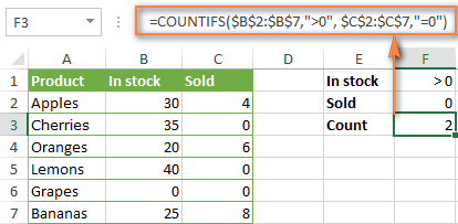
Suppose you have a product list like shown in the screenshot below. You want to get a count of items that are in stock (value in column B is greater than 0) but have not been sold yet (value is column C is equal to 0).
The task can be accomplished by using this formula:
=COUNTIFS(B2:B7,">0", C2:C7,"=0")
And the count is 2 ("Cherries" and "Lemons"):
Formula 2. COUNTIFS formula with two criteria
When you want to count items with identical criteria, you still need to supply each criteria_range / criteria pair individually.
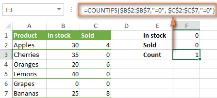
For example, here's the right formula to count items that have 0 both in column B and column C:
=COUNTIFS($B$2:$B$7,"=0", $C$2:$C$7,"=0")
This COUNTIFS formula returns 1 because only "Grapes" have "0" value in both columns.
Using a simpler formula with a single criteria_range like COUNTIFS(B2:C7,"=0") would yield a different result - the total count of cells in the range B2:C7 containing a zero (which is 4 in this example).
How to count cells with multiple criteria (OR logic)
As you have seen in the above examples, counting cells that meet all of the specified criteria is easy because the COUNTIFS function is designed to work this way.
But what if you want to count cells for which at least one of the specified conditions is TRUE, i.e. based on the OR logic? Overall, there are two ways to do this - by adding up several COUNTIF formulas or using a SUM COUNTIFS formula with an array constant.
Formula 1. Add up two or more COUNTIF or COUNITFS formulas
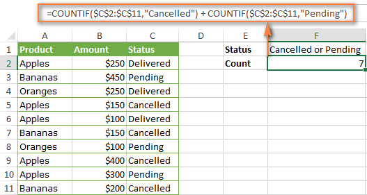
In the table below, supposing you want to count orders with the "Cancelled" and "Pending" status. To have it doen, you can simply write 2 regular Countif formulas and add up the results:
=COUNTIF($C$2:$C$11,"Cancelled") + COUNTIF($C$2:$C$11,"Pending")
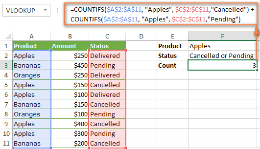
In case each of the functions is supposed to evaluate more than one condition, use COUNTIFS instead of COUNTIF. For example, to get the count of "Cancelled" and "Pending" orders for "Apples" use this formula:
=COUNTIFS($A$2:$A$11, "Apples", $C$2:$C$11,"Cancelled") + COUNTIFS($A$2:$A$11, "Apples", $C$2:$C$11,"Pending")
Formula 2. SUM COUNTIFS with an array constant
In situations when you have to evaluate a lot of criteria, the above approach is not the best way to go because your formula would grow too big in size. To perform the same calculations in a more compact formula, list all of your criteria in an array constant, and supply that array to the criteria argument of the COUNTIFS function. To get the total count, embed COUNTIFS inside the SUM function, like this:
In our sample table, to count orders with the status "Cancelled" or "Pending" or "In transit", the formula would go as follows:
=SUM(COUNTIFS($C$2:$C$11, {"cancelled", "pending", "in transit"}))
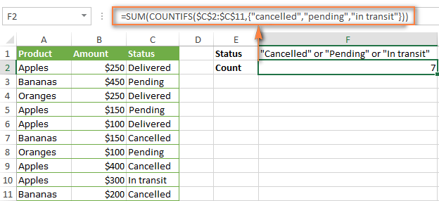
In a similar manner, you can count cells based on two or more criteria_range / criteria pairs. For instance, to get the number of "Apples" orders that are "Cancelled" or "Pending" or "In transit", use this formula:
=SUM(COUNTIFS($A$2:$A$11,"apples",$C$2:$C$11,{"cancelled","pending","in transit"}))

You can find a few more ways to count cells with OR logic in this tutorial: Excel COUNTIF and COUNTIFS with OR conditions.
How to count numbers between 2 specified numbers
By and large, COUNTIFS formulas for numbers fall into 2 categories - based on several conditions (explained in the above examples) and between the two values you specify. The latter can be accomplished in two ways - by using the COUNTIFS function or by subtracting one COUNTIF from another.
Formula 1. COUNTIFS to count cells between two numbers
To find out how many numbers between 5 and 10 (not including 5 and 10) are contained in cells C2 through C10, use this formula:
=COUNTIFS(C2:C10,">5", C2:C10,"<10")
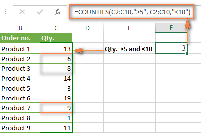
To include 5 and 10 in the count, use the "greater than or equal to" and "less than or equal to" operators:
=COUNTIFS(B2:B10,">=5", B2:B10,"<=10")
Formula 2. COUNTIF formulas to count numbers between X and Y
The same result can be achieved by subtracting one Countif formula from another. The first one counts how many numbers are greater than the lower bound value (5 in this example). The second formula returns the count of numbers that are greater than the upper bound value (10 in this case). The difference between the first and second number is the result you are looking for.
- =COUNTIF(C2:C10,">5")-COUNTIF(C2:C10,">=10") - counts how many numbers greater than 5 and less than 10 are in the range C2:C10. This formula will return the same count as shown in the screenshot above.
- =COUNTIF(C2:C10, ">=5")-COUNTIF(C2:C10, ">10") - the formula counts how many numbers between 5 and 10 are in the range C2:C10, including 5 and 10.
How to use cell references in COUNTIFS formulas
When using logical operators such as ">", "<", "<=" or ">=" together with cell references in your Excel COUNTIFS formulas, remember to enclose the operator in "double quotes" and
add an ampersand (&) before a cell reference to construct a text string.
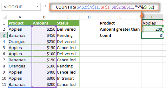
In a sample dataset below, let's count "Apples" orders with amount greater than $200. With criteria_range1 in cells A2:A11 and criteria_range2 in B2:B11, you can use this formula:
=COUNTIFS($A$2:$A$11, "Apples", $B$2:$B$11, ">200")
Or, you can input your criteria values in certain cells, say F1 and F2, and reference those cells in your formula:
=COUNTIFS($A$2:$A$11, $F$1, $B$2:$B$11, ">"&$F$2)
Please notice the use of absolute cell references both in the criteria and criteria_range arguments, which prevents the formula from being broken when copied to other cells.
For more information about the use of an ampersand in COUNTIF and COUNTIFS formulas, please see Excel COUNTIF - frequently asked questions.
How to use COUNTIFS with wildcard characters
In Excel COUNTIFS formulas, you can use the following wildcard characters:
- Question mark (?) - matches any single character, use it to count cells starting and/or ending with certain characters.
- Asterisk (*) - matches any sequence of characters, you use it to count cells containing a specified word or a character(s) as part of the cell's contents.
Tip. If you want to count cells with an actual question mark or asterisk, type a tilde (~) before an asterisk or question mark.
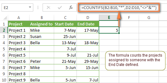
Now let's see how you can use a wildcard char in real-life COUNTIFS formulas in Excel. Suppose, you have a list of projects in column A. You wish to know how many projects are already assigned to someone, i.e. have any name in column B. And because we are learning how to use the COUNTIFS function with multiple criteria, let's add a second condition - the End Date in column D should also be set.
Here is the formula that works a treat:
=COUNTIFS(B2:B10,"*",D2:D10,"<>"&""))
Please note, you cannot use a wildcard character in the 2nd criteria because you have dates rather that text values in column D. That is why, you use the criteria that finds non-blank cells: "<>"&""
COUNTIFS and COUNTIF with multiple criteria for dates
The COUNTIFS and COUNTIF formulas you use for dates are very much similar to the above formulas for numbers.
Example 1. Count dates in a specific date range
To count the dates that fall in a certain date range, you can also use either a COUNTIFS formula with two criteria or a combination of two COUNTIF functions.
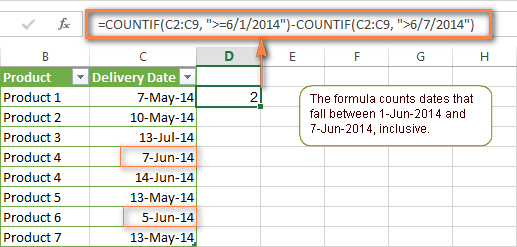
For example, the following formulas count the number of dates in cells C2 through C10 that fall between 1-Jun-2014 and 7-Jun-2014, inclusive:
=COUNTIFS(C2:C9, ">=6/1/2014", C2:C9, "<=6/7/2014")
=COUNTIF(C2:C9, ">=6/1/2014") - COUNTIF(C2:C9, ">6/7/2014")
Example 2. Count dates with multiple conditions
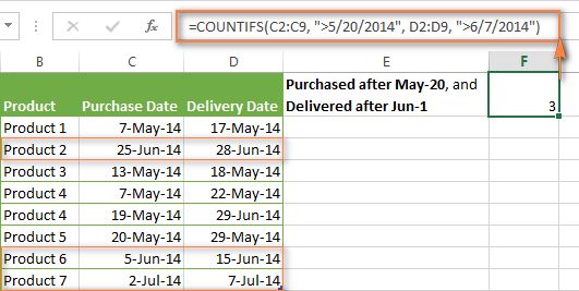
In the same manner, you can use a COUNTIFS formula to count the number of dates in different columns that meet 2 or more conditions. For instance, the below formula will find out how many products were purchased after the 20th of May and delivered after the 1st of June:
=COUNTIFS(C2:C9, ">5/1/2014", D2:D9, ">6/7/2014")
Example 3. Count dates with multiple conditions based on the current date
You can use Excel's TODAY() function in combination with COUNTIF to count dates based on the current date.
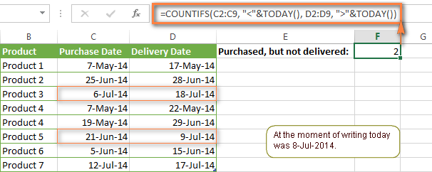
For example, the following COUNTIF formula with two ranges and two criteria will tell you how many products have already been purchased but not delivered yet.
=COUNTIFS(C2:C9, "<"&TODAY(), D2:D9, ">"&TODAY())
This formula allows for many possible variations. For instance, you can tweak it to count how many products were purchased more than a week ago and are not delivered yet:
=COUNTIFS(C2:C9, "<="&TODAY()-7, D2:D9, ">"&TODAY())
This is how you count cells with multiple criteria in Excel. I hope you will find these examples helpful. Anyway, I thank you for reading and hope to see you on our blog next week!
 by
by
2035 comments
Excellent! Thanks for the clear explanation. This really helped.
H
Hi Alexander,
I guess even my query has been missed out. 176 is my number. So please if you can help me out.
Thank you.
I have two columns, column 1- Dates, column 2- Names.
01/02/2015 ARYA
01/02/2015 ARYA
01/02/2015 ARYA
02/02/2015 ARYA
From the above example, I want the count to reflect 2, in other words I would want it to count as a single occurrence per day i.e., 01/02 - one occurrence & 02/02 one occurrence. Please help me with this. Please help me without date ranges as i need to use it for the entire year for different names.
Hello there, I hope you can help with the following worksheet with multiple tabs.I Maybe COUNTIF could work but i really can't figure it out how.
Code Account Title Jan-05 Feb-05
1000 Advertising $750,75 $-
2000 Office Equipment $- $-
3000 Printers $- $-
1st- I would like to set the date in each column as 16Jan-15Feb, 16Feb-15Mar etc., so that it sums up the invoices amount for each code of only those dates, at the moment it only adds each full month, and i can't seem to find a way to change it without errors. This is how the formula is shown:
=SUMIF('Itemized Expenses'!$J:$J;"="&($A6&TEXT(C$4;"mmm-yy"));'Itemized Expenses'!$E:$E
2nd - I would like to add another formula to this, which also adds the amounts within those dates depending on methods of payment and display it in another column, that is the total paid in cash, total credit card, total direct debit, etc.
Thank you very much in advance for your help.
Lotus
I am ubable to count below data
Name Time
A 12:03:00 PM
B 12:17:00 PM
C 12:00:00 PM
D 12:44:00 PM
E 5:01:00 PM
f 12:21:00 PM
A 12:03:00 PM
B 12:17:00 PM
C 12:00:00 PM
D 12:44:00 PM
E 5:01:00 PM
f 12:21:00 PM
A 12:03:00 PM
B 12:17:00 PM
C 12:00:00 PM
D 12:44:00 PM
E 5:01:00 PM
f 12:21:00 PM
NAME Count
A
B
C
D
E
f
Please help
Thanks again Alexander.
Thanks Alexander, but the formula counts empty cells also in the column. How to count only the cells with values, neglecting empty cells?
=SUM(LEN(A2:A10)-LEN(SUBSTITUTE(A2:A10,",",""))+(--NOT(ISBLANK(A2:A10))))
How do you count two different 'tasks' that are in the same column but only if they are marked 'active' in another column.
I seem to have botched this up & have ended up with this mess:
=COUNT((IF('Combined Project & Milestone'!F:G,"DESTRUCTIVE TESTING")),+OR((COUNTIF('Combined Project & Milestone'!F:G,"INITIAL REPORT")),+(COUNTIF('Combined Project & Milestone'!F:G,"Active"))))
REALLY hope you can help soon.
Thanks
Please disregard the above - I worked it out.
How to count the number of values in a cells separated with a coma.
eg.
1
4,5
6
The number of values should be 4 in the 3 cells. Count function only counts 2 values.
Please use this array formula (press Ctrl+Shift+Enter to complete it):
=SUM(LEN(A2:A10)-LEN(SUBSTITUTE(A2:A10,",",""))+1)
Where A2:A10 is your cells with data. Please note that the formula will return wrong results, if your cells contain some text, e.g. "1,text,text20"
Hi,I Am making a file for my poject.I am facing the some problem in xls pls do help in that. I have to add the farmula that How may rows is on Time and Early only for NAGAR as given the example. total should be come in one cell for both On time+Early of the NAGAR name.
NAGAR On Time
RPRAD Early
BBIAD Late
CCUBG Late
NAGAR On Time
RPRAD Late
BBIAD Late
CCUBG Late
NAGAR Early
RPRAD Early
BBIAD Early
CCUBG Early
NAGAR On Time
RPRAD Early
BBIAD Late
CCUBG Late
NAGAR Early
RPRAD On Time
BBIAD Late
CCUBG Late
NAGAR On Time
RPRAD Late
BBIAD Late
CCUBG Late
Thank you.
Please use
=countifs(A2:A1000, "NAGAR", B2:B1000, "On Time") + countifs(A2:A1000, "NAGAR", B2:B1000, "Early")
Grate. Thank You.....
Thanks Svetlana, you just saved my life and a lot of typing :) awesome post
1 JAMES SHJ MALE MALE FEMALE KIDS
2 RICKY DXB MALE SHJ Formula ? Formula ? Formula ? 7
3CHRISTINA SHJ FEMALE DXB Formula ? Formula ? Formula ? 2
4 LIBA SHJ KIDS AUH Formula ? Formula ? Formula ? 2
5 JOSEPH AUH MALE 11
6 ZARINA SHJ FEMALE
7 WINSTON DXB MALE
8 JENNIFER SHJ FEMALE
9 MINNU SHJ KIDS
10 ARASH AUH MALE
11 MAHIR SHJ MALE
uum yeah, that was very clear how's going to Dubai and sharjah I suppose?
Hello Eddie,
I am sorry, your data look distorted in the comment. For us to be able to assist you better, please post a small sample workbook with your data on our forums and describe in detail what you want to count. We will try to help.
I've been reading around and I apologize if I've missed this(the information has me a bit...confused and I overwhelmed)
I am trying to keep track of some projects between me and a person.
Under one column of cells I have the type of project and in another I have who did it.
I have somewhere a list of how many of each TYPE of project is done and beside that who it was done by so I can keep track of the giant project list.
So say...the C columne says "Project type 1" or "Project type 2" and the D column has "Done by Susy" or "Done by Dave"
I was keeping track of "Project type 1" in one cell. So it's counting how many we did of that type very well.
Then I did the same for Project type 2.
But when I got to the point of: "Project type 1 done by Susy", I tried to put in a formula to count how many times Project1 was done by Susy and another counting how many times it was done by Dave.
...cept it doesnt work. And I'm not quite sure how to do it. I got confused reading the information because it seems to always be consistent info in different columns or different info in the same column and rarely did I find "Only count if both these conditions are met"
Is that..even possible? Neither have value numbers. They use words rather than numbers(obviously they arent actually called 'Project 1' and '2'.
Gah..just writing gets me confused.
Hello, i thank you for helping others unconditionally. I have asked for help and posted twice. Number 177 is the only one i can find. I understand that you have extremely high traffic volumne. But i was just wondering if i am able to get help here or even my request for help is misssed. thank you again for the good works you are doing for all persons and society.
I'm trying to calculate the total number of individuals who meet a certain criteria, but I can't seem to make the "COUNTIFS" formula fit what need. I have a column, EDU and here is some sample data. I want all data to count as 1 except "HS" which should not be counted. The purpose is to calculate the number of individuals who have post-HS education.
Do you have suggestions on how to make the formula work with multiple conditions?
EDU
HS
BA
BS
AA
AS
HS
HS
BA
AA
Hello Shannon,
Please use the following formula:
=COUNTA(A2:A20)-COUNTIF(A2:A20,"HS")
Where A2:A10 is the EDU column
Hi! For my previous question I get answer! But I have other one - if I want to count only "OK" results for IF function for example H7:H19, what function do I need to use?
=IF(C7>0;"OK";"BAD") this one is working, but if I put region
=IF(C7:G7>0;"OK";"BAD")or =IF((C7:G7)>0;"OK";"BAD") excel give me VALUE
Hi,
I'm trying to get excel to find numbers ending in a 7 (i.e. 47, 57, 67) and then need to tell the computer is raise the number to 47 to 50, 57 to 60 and 67 to 70. Please can someone help please?
Thanks
Sue
Hi Svetlana,
I hope you may be able to help?1?
I am designing an attendance spreadsheet for a school using a set of alphabetic codes for attendance, for example - P- Attended, L - Half day, A - Absent.
I also have a summary box for reporting purposes and need to count attendance and absence based on gender (M/F) and grade(k - 10) and ethic background (I,NI) (a column for each).
Therefore I need to count the number of Ps, or A's that exists in the attendance data in the row IF gender=M and grade=K and ethnicity=I
I also want a value returned if the cell is still empty.
I am have tried using : =COUNT(IF((C6:C19="K")*(E6:E19="M"),F6:BM19="P"))
But this returns will a nil value.
Let me know if I need to send through the spreadsheet.
Thanks in anticipation.
Jessie
Warm regards,
Jessie
DATE Service sum(totalHits) sum(Successful) sum(Dispatched) sum(Failed)
11/1/2014 MPESA Uploader 373 285 =COUNTIF:(sheet1:status1,"<=103", sheet1:status1,"<=202")
11/2/2014 MPESA Uploader 227 158 1
11/3/2014 MPESA Uploader 285 284 1
11/4/2014 MPESA Uploader 294 294 0
11/5/2014 MPESA Uploader 301 301 0
11/6/2014 MPESA Uploader 253 251 2
11/7/2014 MPESA Uploader 274 273 1
11/8/2014 MPESA Uploader 283 281 2
11/9/2014 MPESA Uploader 2 2 0
11/10/2014 MPESA Uploader 268 268 0
11/11/2014 MPESA Uploader 7 7 0
11/12/2014 MPESA Uploader 58 57 1
11/13/2014 MPESA Uploader 243 243 0
11/14/2014 MPESA Uploader 195 195 0
11/15/2014 MPESA Uploader 259 259 0
11/16/2014 MPESA Uploader 299 296 3
11/17/2014 MPESA Uploader 291 289 2
11/18/2014 MPESA Uploader 342 342 0
11/19/2014 MPESA Uploader 335 335 0
11/20/2014 MPESA Uploader 394 393 1
11/21/2014 MPESA Uploader 304 302 2
11/22/2014 MPESA Uploader 295 295 0
11/23/2014 MPESA Uploader 308 308 0
11/24/2014 MPESA Uploader 625 617 8
11/25/2014 MPESA Uploader 361 361 0
11/26/2014 MPESA Uploader 295 295 0
11/27/2014 MPESA Uploader 356 356 0
11/28/2014 MPESA Uploader 262 262 0
11/29/2014 MPESA Uploader 227 227 0
11/30/2014 MPESA Uploader 358 358 0
I need to compute the sum failed