The tutorial provides a list of Excel basic formulas and functions with examples and links to related in-depth tutorials.
Being primarily designed as a spreadsheet program, Microsoft Excel is extremely powerful and versatile when it comes to calculating numbers or solving math and engineering problems. It enables you to total or average a column of numbers in the blink of an eye. Apart from that, you can compute a compound interest and weighted average, get the optimal budget for your advertising campaign, minimize the shipment costs or make the optimal work schedule for your employees. All this is done by entering formulas in cells.
This tutorial aims to teach you the essentials of Excel functions and show how to use basic formulas in Excel.
The basics of Excel formulas
Before providing the basic Excel formulas list, let's define the key terms just to make sure we are on the same page. So, what do we call an Excel formula and Excel function?
- Formula is an expression that calculates values in a cell or in a range of cells.
For example,
=A2+A2+A3+A4is a formula that adds up the values in cells A2 through A4. - Function is a predefined formula already available in Excel. Functions perform specific calculations in a particular order based on the specified values, called arguments, or parameters.
For example, instead of specifying each value to be summed like in the above formula, you can use the SUM function to add up a range of cells: =SUM(A2:A4)
You can find all available Excel functions in the Function Library on the Formulas tab:

There exist 400+ functions in Excel, and the number is growing by version to version. Of course, it's next to impossible to memorize all of them, and you actually don't need to. The Function Wizard will help you find the function best suited for a particular task, while the Excel Formula Intellisense will prompt the function's syntax and arguments as soon as you type the function's name preceded by an equal sign in a cell:
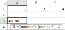
Clicking the function's name will turn it into a blue hyperlink, which will open the Help topic for that function.
Tip. You don't necessarily have to type a function name in all caps, Microsoft Excel will automatically capitalize it once you finish typing the formula and press the Enter key to complete it.
10 Excel basic functions you should definitely know
What follows below is a list of 10 simple yet really helpful functions that are a necessary skill for everyone who wishes to turn from an Excel novice to an Excel professional.
SUM
The first Excel function you should be familiar with is the one that performs the basic arithmetic operation of addition:
In the syntax of all Excel functions, an argument enclosed in [square brackets] is optional, other arguments are required. Meaning, your Sum formula should include at least 1 number, reference to a cell or a range of cells. For example:
=SUM(B2:B6) - adds up values in cells B2 through B6.
=SUM(B2, B6) - adds up values in cells B2 and B6.
If necessary, you can perform other calculations within a single formula, for example, add up values in cells B2 through B6, and then divide the sum by 5:
=SUM(B2:B6)/5
To sum with conditions, use the SUMIF function: in the 1st argument, you enter the range of cells to be tested against the criteria (A2:A6), in the 2nd argument - the criteria itself (D2), and in the last argument - the cells to sum (B2:B6):
=SUMIF(A2:A6, D2, B2:B6)
In your Excel worksheets, the formulas may look something similar to this:

Tip. The fastest way to sum a column or row of numbers is to select a cell next to the numbers you want to sum (the cell immediately below the last value in the column or to the right of the last number in the row), and click the AutoSum button on the Home tab, in the Formats group. Excel will insert a SUM formula for you automatically.
Useful resources:
AVERAGE
The Excel AVERAGE function does exactly what its name suggests, i.e. finds an average, or arithmetic mean, of numbers. Its syntax is similar to SUM's:
Having a closer look at the formula from the previous section (=SUM(B2:B6)/5), what does it actually do? Sums values in cells B2 through B6, and then divides the result by 5. And what do you call adding up a group of numbers and then dividing the sum by the count of those numbers? Yep, an average!
The Excel AVERAGE function performs these calculations behind the scenes. So, instead of dividing sum by count, you can simply put this formula in a cell:
=AVERAGE(B2:B6)
To average cells based on condition, use the following AVERAGEIF formula, where A2:A6 is the criteria range, D3 is he criteria, and B2:B6 are the cells to average:
=AVERAGEIF(A2:A6, D3, B2:B6)

Useful resources:
MAX & MIN
The MAX and MIN formulas in Excel get the largest and smallest value in a set of numbers, respectively. For our sample data set, the formulas will be as simple as:
=MAX(B2:B6)
=MIN(B2:B6)

Useful resources:
COUNT & COUNTA
If you are curious to know how many cells in a given range contain numeric values (numbers or dates), don't waste your time counting them by hand. The Excel COUNT function will bring you the count in a heartbeat:
While the COUNT function deals only with those cells that contain numbers, the COUNTA function counts all cells that are not blank, whether they contain numbers, dates, times, text, logical values of TRUE and FALSE, errors or empty text strings (""):
For example, to find out how many cells in column B contain numbers, use this formula:
=COUNT(B:B)
To count all non-empty cells in column B, go with this one:
=COUNTA(B:B)
In both formulas, you use the so-called "whole column reference" (B:B) that refers to all the cells within column B.
The following screenshot shows the difference: while COUNT processes only numbers, COUNTA outputs the total number of non-blank cells in column B, including the the text value in the column header.

Useful resources:
IF
Judging by the number of IF-related comments on our blog, it's the most popular function in Excel. In simple terms, you use an IF formula to ask Excel to test a certain condition and return one value or perform one calculation if the condition is met, and another value or calculation if the condition is not met:
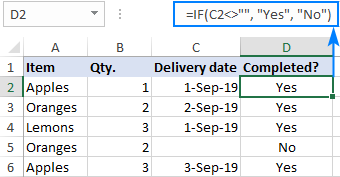
For example, the following IF statement checks if the order is completed (i.e. there is a value in column C) or not. To test if a cell is not blank, you use the "not equal to" operator ( <>) in combination with an empty string (""). As the result, if cell C2 is not empty, the formula returns "Yes", otherwise "No":
=IF(C2<>"", "Yes", "No")
Useful resources:
TRIM
If your obviously correct Excel formulas return just a bunch of errors, one of the first things to check is extra spaces in the referenced cells (You may be surprised to know how many leading, trailing and in-between spaces lurk unnoticed in your sheets just until something goes wrong!).
There are several ways to remove unwanted spaces in Excel, with the TRIM function being the easiest one:
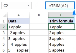
For example, to trim extra spaces in column A, enter the following formula in cell A1, and then copy it down the column:
=TRIM(A1)
It will eliminate all extra spaces in cells but a single space character between words:
Useful resources:
LEN
Whenever you want to know the number of characters in a certain cell, LEN is the function to use:
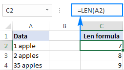
Wish to find out how many characters are in cell A2? Just type the below formula into another cell:
=LEN(A2)
Please keep in mind that the Excel LEN function counts absolutely all characters including spaces:
Want to get the total count of characters in a range or cells or count only specific characters? Please check out the following resources.
Useful resources:
AND & OR
These are the two most popular logical functions to check multiple criteria. The difference is how they do this:
- AND returns TRUE if all conditions are met, FALSE otherwise.
- OR returns TRUE if any condition is met, FALSE otherwise.
While rarely used on their own, these functions come in very handy as part of bigger formulas.
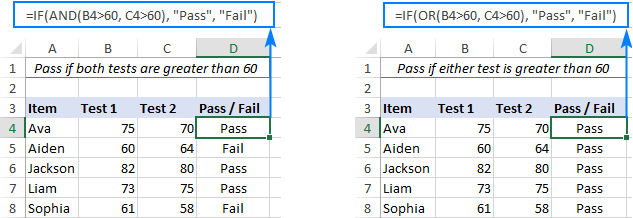
For example, to check the test results in columns B and C and return "Pass" if both are greater than 60, "Fail" otherwise, use the following IF formula with an embedded AND statement:
=IF(AND(B2>60, B2>60), "Pass", "Fail")
If it's sufficient to have just one test score greater than 60 (either test 1 or test 2), embed the OR statement:
=IF(OR(B2>60, B2>60), "Pass", "Fail")
Useful resources:
CONCATENATE
In case you want to take values from two or more cells and combine them into one cell, use the concatenate operator (&) or the CONCATENATE function:
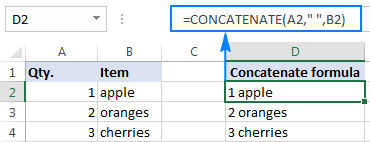
For example, to combine the values from cells A2 and B2, just enter the following formula in a different cell:
=CONCATENATE(A2, B2)
To separate the combined values with a space, type the space character (" ") in the arguments list:
=CONCATENATE(A2, " ", B2)
Useful resources:
TODAY & NOW
To see the current date and time whenever you open your worksheet without having to manually update it on a daily basis, use either:
=TODAY() to insert the today's date in a cell.
=NOW() to insert the current date and time in a cell.
The beauty of these functions is that they don't require any arguments at all, you type the formulas exactly as written above.

Useful resources:
Best practices for writing Excel formulas
Now that you are familiar with the basic Excel formulas, these tips will give you some guidance on how to use them most effectively and avoid common formula errors.
Do not enclose numbers in double quotes
Any text included in your Excel formulas should be enclosed in "quotation marks". However, you should never do that to numbers, unless you want Excel to treat them as text values.
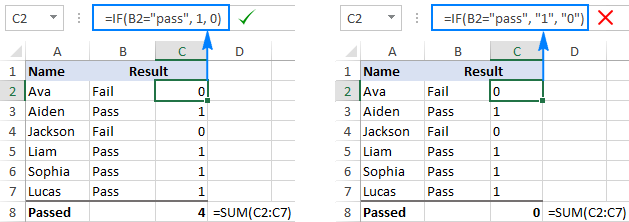
For example, to check the value in cell B2 and return 1 for "Passed", 0 otherwise, you put the following formula, say, in C2:
=IF(B2="pass", 1, 0)
Copy the formula down to other cells and you will have a column of 1's and 0's that can be calculated without a hitch.
Now, see what happens if you double quote the numbers:
=IF(B2="pass", "1", "0")
At first sight, the output is normal - the same column of 1's and 0's. Upon a closer look, however, you will notice that the resulting values are left-aligned in cells by default, meaning those are numeric strings, not numbers! If later on someone will try to calculate those 1's and 0's, they might end up pulling their hair out trying to figure out why a 100% correct Sum or Count formula returns nothing but zero.
Don't format numbers in Excel formulas
Please remember this simple rule: numbers supplied to your Excel formulas should be entered without any formatting like decimal separator or dollar sign. In North America and some other countries, comma is the default argument separator, and the dollar sign ($) is used to make absolute cell references. Using those characters in numbers may just drive your Excel crazy :) So, instead of typing $2,000, simply type 2000, and then format the output value to your liking by setting up a custom Excel number format.
Match all opening and closing parentheses
When crating a complex Excel formula with one or more nested functions, you will have to use more than one set of parentheses to define the order of calculations. In such formulas, be sure to pair the parentheses properly so that there is a closing parenthesis for every opening parenthesis. To make the job easier for you, Excel shades parenthesis pairs in different colors when you enter or edit a formula.
Copy the same formula to other cells instead of re-typing it
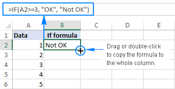
Once you have typed a formula into a cell, there is no need to re-type it over and over again. Simply copy the formula to adjacent cells by dragging the fill handle (a small square at the lower right-hand corner of the cell). To copy the formula to the whole column, position the mouse pointer to the fill handle and double-click the plus sign.
Note. After copying the formula, make sure that all cell references are correct. Cell references may change depending on whether they are absolute (do not change) or relative (change).
For the detailed step-by-step instructions, please see How to copy formulas in Excel.
How to delete formula, but keep calculated value
When you remove a formula by pressing the Delete key, a calculated value is also deleted. However, you can delete only the formula and keep the resulting value in the cell. Here's how:
- Select all cells with your formulas.
- Press Ctrl + C to copy the selected cells.
- Right-click the selection, and then click Paste Values > Values to paste the calculated values back to the selected cells. Or, press the Paste Special shortcut: Shift+F10 and then V.
For the detailed steps with screenshots, please see How to replace formulas with their values in Excel.
Make sure Calculation Options are set to Automatic
If all of a sudden your Excel formulas have stopped recalculating automatically, most likely the Calculation Options somehow switched to Manual. To fix this, go to the Formulas tab > Calculation group, click the Calculation Options button, and select Automatic.
If this does not help, check out these troubleshooting steps: Excel formulas not working: fixes & solutions.
This is how you make and manage basic formulas in Excel. I how you will find this information helpful. Anyway, I thank you for reading and hope to see you on our blog next week.
 by
by
409 comments
its very informative and Thanx for this ..
any body have any other formula regarding excel kindly mail me or whatsapp
It's was to help ful to me
how to fetch one table to another table data
Say
buyer X received 123 pcs from unit 1
buyer X received 500 pcs from unit 2
buyer X received 280 pcs from unit 3
buyer y received 123 pcs from unit 3
buyer y received 123 pcs from unit 1
buyer Z received 123 pcs from unit 2
buyer Z received 123 pcs from unit 1
Please put formula who I calculate buyer wise and unit wise received total qty
Give me the formula name for
C3*C4%+C3
Very good
Can u teach us how to make general ledger tria balance
SR NO FORUMAULA
IF I HAVE TWO COLOMS A & B WHERE "A" HAS MATERIAL AND "B" HAS QTY. AND DON'T WANT TO FILTER TO COUNT PARTICULAR QTY FOR MATERIAL ,SO I WILL DO WORK IN A NEW COLOM "D" AS MATERIAL AND "E" QTY AND WHAT I NEED HELP THAT AUTOMATICALLY QTY ADD UP IN COLOM "D" & "E" WHEN I WILL DO ENTRY IN "A" & "B"..PLEASE REVERT ME IF YOU NEED SCREEN SHOT OF MY WORK...
nice explanation
if Total cost is 10000. i want to calculate what is the value which includes 12% in 10000. Tell me the formula pl.
ex: TOTAL COST A1
PRICE :=A1*100/112
REALLY VERY HELPFUL THANKU
=num2text FIGURES TO WORDS
Hello,
I have been asked to extract the number from the following list without using MID as this only works when all the results are the same type.
TX TO 2014016 CHG ORG
TX TO 1832298CHG ORG DEN
TX TO 1854600 CHG ORG
TX TO 1971447
TX TO 1980547 CHG ORG
Any help is appreciated
Hello,
If you need to avoid using the MID function to fulfill your task, then I can recommend you to try extracting numbers from your list of data with the help of the Extract Text tool.
I sew and i believe about all form A.I.A
Do data jaise colume A or colume B dono ka data colume A me Lana hai to kon SA formula use hoga
K L
COLUMN COLUMN
R M =CONCATENATE(K15," ",L15)
= R M
= " " STANDS FOR SPACE
Qut Amount Discount Amount
2 300 20% ===
THANKS YOU
Sum (no1, no 2)
if sheet 1 - particular cell value is visible in sheet 2 - What is the formula for that?
Deduction under VI A in incometax calulation is 150000 but Candidate Have Deduction more then 150000 or Less than 150000 we want to rebate only 150000 what is the formula in exel
Sorry, my typing was inaccurate, the first column should be Monthly Basic Salary x 2.75% with values that ranges from P10,000 to P40,000. The second column should be Monthly Premium with values P275, P275.02-P1,099.99 & P1,100.
Hope this is clear now.
Thanks
Hello,
Supposing that your table starts from A1, please try to do the following:
1. Enter P10,000.00 in cell A2;
2. Enter the following formula in cell B2:
=A2*2.75%
3. Select the cells with your data and drag the fill handle (a small square at the lower right-hand corner of the selected cell) down.
Hope it will help you.
Hi, can you help me create a formula for below table? I have tried but there is lacking in result for the condition of P40,000 and above.
Monthly Basic Monthly
Salary x 2.75% Premium
P10,000.00 & below P275
P10,000.01-P39,999.99 P275.02-P1,099.99
P40,000.00 & above P1,100.00
Thank you in advance.
explain excel
Hi, I need to calculate % discount in my spreadsheet, I need a kind assistance. Thanks.
Hello,
For me to understand the problem better, please send me a small sample workbook with your source data and the result you expect to get to support@ablebits.com. Please don't worry if you have confidential information there, we never disclose the data we get from our customers and delete it as soon as the problem is resolved.
Please also don't forget to include the link to this comment into your email.
I'll look into your task and try to help.
dear concern:
in excel i cant correct the below function .please help me
04KRKKRK i want to delete 04KRK AD ADD 04BNUKRK at whole list.plz
04KRKKRK
04KRKKRK
04KRKKRK
04KRKKRK
up to 1000
A B C D
04KRKKRK =LEFT(3,A1) YOURWRLD =B1&""&C1 (COPY THAT IN ALL CELL)
04KRKKRK
04KRKKRK
HELLO..can anyone help me using formulas in payroll?
heres the data summary example:
name rate/mo deductions total net
sss phic hdmf deductions pay
1) A 13000 1200 125 500 1825 11175
2) B 25000 1700 125 1000 2825 22175
what i want is in a certain payslip i just encode #1 then all the details will come out in just one click...is it possible?
thank u for the guidance.
Hello,
For me to understand the problem better, please send me a small sample workbook with your source data and the result you expect to get to support@ablebits.com. Please don't worry if you have confidential information there, we never disclose the data we get from our customers and delete it as soon as the problem is resolved.
Please also don't forget to include the link to this comment into your email.
I'll look into your task and try to help.
At first you must have the time of particular date then can find through apply below formula.
=int(time-date)
Hello,
Can anyone tell me how can I calculate elapsed days if I have a date & time in place.
such as I want to calculate how much time has been elapsed till this time from the given date & time.
2017-11-13 19:35:19
Hello,
Please try the following formula:
=DATEDIF(A1,IF(TIME(HOUR(A1),MINUTE(A1), SECOND(A1))> TIME(HOUR(NOW()),MINUTE(NOW()),SECOND(NOW())),NOW()-1,NOW()),"D")&" days "&HOUR((1-VALUE(TIME(HOUR(A1),MINUTE(A1), SECOND(A1))))+ VALUE(TIME(HOUR(NOW()), MINUTE(NOW()), SECOND(NOW()))))&" hours "&MINUTE((1-VALUE(TIME(HOUR(A1),MINUTE(A1),SECOND(A1))))+ VALUE(TIME(HOUR(NOW()),MINUTE(NOW()),SECOND(NOW()))))&" minutes "&SECOND((1-VALUE(TIME(HOUR(A1), MINUTE(A1), SECOND(A1))))+ VALUE(TIME(HOUR(NOW()), MINUTE(NOW()), SECOND(NOW()))))&" seconds"
Hope it will help you.
Great Dear But it is Not Automatic I have to refresh then it will work please do work for this Automatic Running line Hours Mints and secound
Please what does this formula mean in a sentence form?
=RANK(A2,A$2:A$8)&MID("thstndrdth",MIN(9,2*RIGHT(RANK(A2,A$2:A$8))*(MOD(RANK(A2,A$2:A$8)-11,100)>2)+1),2)
Hi, I want to know what vlookup can use in "if". Means it the condition is true then vlookup will run.
Hi Babu,
You can nest a Vlookup formula in the value_if_true argument of the IF function like this:
=IF(logical_test, VLOOKUP(...), "")
Plese send the transfer to number in word formula
good
=IF(COUNTIF(A2:E2,"0")=5, "STRONG", IF(COUNTIF(A2:E2,"0")=4,"GOOD",IF(COUNTIF(A2:E2,"0")=3, "POSITIVE","WEAK")))
if in sheet 1 there is a roll no of student in A1 and class in B1. I want that I write roll no in sheet 2 A1 and class automatically written in sheet 2
Hello, Shakeel,
I'm afraid there's no easy way to solve your task with a formula. Using a VBA macro would be the best option here.
However, since we do not cover the programming area (VBA-related questions), I can advice you to try and look for the solution in VBA sections on mrexcel.com or excelforum.com.
Sorry I can't assist you better.
Woww. I have learnt Excel...
plz give me all excel forumullas
Pls give me excell formulas with example i need ......
Thank you
Excel Is Mathematical App So We Need More Explanation About Ms~excel
Hi there!
You can use the following formula:
=IF(COUNTIF(A2:E2,">0")=5,"STRONG", IF(COUNTIF(A2:E2,">0")=4,"GOOD", IF(COUNTIF(A2:E2,">0")=3,"POSITIVE","WEAK")))
Hope this will help you :)
thanks that was so useful for me!
please send all excel formulas with explanation for both windows and apple iOS
Hello,
you can see the full list of all the Excel functions on this web-page. They can be used in both, Windows and Mac.
If you want to improve your knowledge of Excel formulas and functions, you can subscribe to our blog feed by clicking on the "Register" link on the right side of this page.
Every week we post different tips and tricks on our blog that will help you to solve every-day tasks in Excel.
Hope you will find this information helpful.
Hi Svetlana,
I am working percentage. here's my need. I must calculate 5% of a sum but there's a cap for eg.
5% of 125,000 = 6,250 (this is the ceiling)
if the sum increases to 130,000 the ceiling can't be exceeded.
So I need a formula to tell the cell to calculate 5% of the particular amount up to 125,000 but apply the ceiling of 6250 whenever 125,000 is exceeded.
Hope I explained simply enough.
Thank you!
Easiest way is to use an IF Function:
=if(A1<=125000,A1*.05,6250)
In this case, A1 is the sum you are trying to multiply by 5%
I think you are just trying to act smart
Thank you friend
Hi,
How to highlight the value in a cell whenever which is higher than that of in the preceding cell? Is such function found in conditional formatting?
12.94 12.94 13.00 12.93 12.92 12.91 12.9 12.89 12.89 12.9 12.89
Thanks.
madam
excel if, else condition formala example sent my email id
Hey there,
I want one formula wherein,
A B C D E
1 0 2 4 5
If all of the above columns are greater than 0 then result would be "STRONG", If any 4 of the above columns are greater than 0 then the result would be "GOOD" and if any 3 of the above columns are greater than 0 then result would be "POSITIVE" otherwise it would be "WEAK".
It would be really great if you may help in this.
Thanks & regards,
Ankita Matalia
Hi there!
You can use the following formula:
=IF(COUNTIF(A2:E2,">0")=5,"STRONG",IF(COUNTIF(A2:E2,">0")=4,"GOOD",IF(COUNTIF(A2:E2,">0")=3,"POSITIVE","WEAK")))
Hope this will help you :)
good
ms excle all formula list
Thank's Svetlana.