The tutorial explains the MAX function with many formula examples that show how to find highest value in Excel and highlight largest number in your worksheet.
MAX is one of the most straightforward and easy-to-use Excel functions. However, it does have a couple of tricks knowing which will give you a big advantage. Say, how do you use the MAX function with conditions? Or how would you extract the absolute largest value? This tutorial provides more than one solution for these and other related tasks.
Excel MAX function
The MAX function in Excel returns the highest value in a set of data that you specify.
The syntax is as follows:
Where number can be represented by a numeric value, array, named range, a reference to a cell or range containing numbers.
Number1 is required, number2 and subsequent arguments are optional.
The MAX function is available in all versions of Excel for Office 365, Excel 2019, Excel 2016, Excel 2013, Excel 2010, Excel 2007, and lower.
How to make a MAX formula in Excel
To create a MAX formula in its simplest from, you can type numbers directly in the list of arguments, like this:
=MAX(1, 2, 3)
In practice, it's quite a rare case when numbers are "hardcoded". For the most part, you will deal with ranges and cells.
The fastest way to build a Max formula that finds the highest value in a range is this:
- In a cell, type =MAX(
- Select a range of numbers using the mouse.
- Type the closing parenthesis.
- Press the Enter key to complete your formula.
For example, to work out the largest value in the range A1:A6, the formula would go as follows:
=MAX(A1:A6)
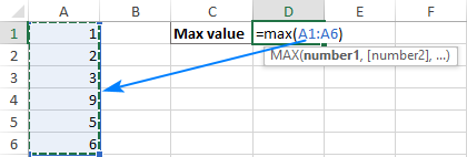
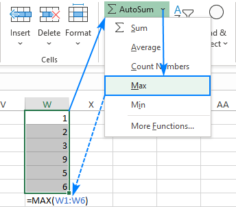
If your numbers are in a contiguous row or column (like in this example), you can get Excel to make a Max formula for you automatically. Here's how:
- Select the cells with your numbers.
- On the Home tab, in the Formats group, click AutoSum and pick Max from the drop-down list. (Or click AutoSum > Max on the Formulas tab in the Function Library group.)
This will insert a ready-to-use formula in a cell below the selected range, so please make sure there is at least one blank cell underneath the list of numbers that you've selected:
5 things to know about MAX function
To successfully use Max formulas your worksheets, please remember these simple facts:
- In the current versions of Excel, a MAX formula can accept up to 255 arguments.
- If the arguments do not contain a single number, the MAX function returns zero.
- If the arguments contain one or more error values, an error is returned.
- Empty cells are ignored.
- Logical values and text representations of numbers supplied directly in the list of arguments are processed (TRUE evaluates as 1, FALSE evaluates as 0). In references, logical and text values are ignored.
How to use MAX function in Excel – formula examples
Below you will find a few typical uses of the Excel MAX function. In many cases, there are a few different solutions for the same task, so I encourage you to test all the formulas to choose the one best suited for your data type.
How to find max value in a group
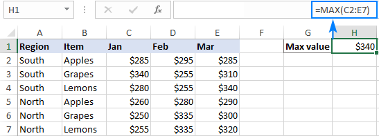
To extract the largest number in a group of numbers, supply that group to the MAX function as a range reference. A range can contain as many rows and columns as you desire. For example, to get the highest value in the range C2:E7, use this simple formula:
=MAX(C2:E7)
Find highest value in non-adjacent cells or ranges
To make a MAX formula for non-contiguous cells and ranges, you need to include a reference to each individual cell and/or range. The following steps will help you to do that quickly and flawlessly:
- Start typing a Max formula in a cell.
- After you've typed the opening parenthesis, hold down the Ctrl key and select the cells and ranges in the sheet.
- After selecting the last item, release Ctrl and type the closing parenthesis.
- Press Enter.
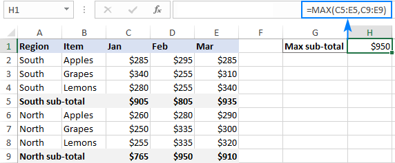
Excel will use an appropriate syntax automatically, and you will get a formula similar to this:
=MAX(C5:E5, C9:E9)
As shown in the screenshot below, the formula returns the maximum sub-total value from rows 5 and 9:
How to get max (latest) date in Excel
In the internal Excel system, dates are nothing else but serial numbers, so the MAX function handles them without a hitch.
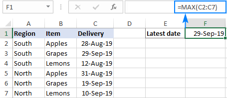
For instance, to find the latest delivery date in C2:C7, make a usual Max formula that you'd use for numbers:
=MAX(C2:C7)
MAX function in Excel with conditions
When you wish to get the maximum value based on conditions, there are several formulas for you to choose from. To make sure that all the formulas return the identical result, we will test them on the same set of data.
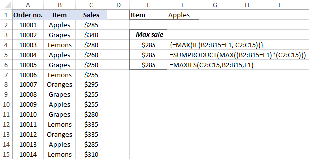
The task: With the items listed in B2:B15 and sales figures in C2:C15, we aim to find the highest sale for a specific item input in F1 (please see the screenshot at the end of this section).
Excel MAX IF formula
If you a looking for a formula that works in all versions of Excel 2000 through Excel 2019, use the IF function to test the condition, and then pass the resulting array to the MAX function:
=MAX(IF(B2:B15=F1, C2:C15))
For the formula to work, it must press Ctrl + Shift + Enter simultaneously to enter it as an array formula. If all done correctly, Excel will enclose your formula in {curly braces}, which is a visual indication of an array formula.
It is also possible to evaluate several conditions in a single formula, and the following tutorial shows how: MAX IF with multiple conditions.
Non-array MAX IF formula
If you don't like using array formulas in your worksheets, then combine MAX with the SUMPRODUCT function that processes arrays natively:
=SUMPRODUCT(MAX((B2:B15=F1)*(C2:C15)))
For more information, please see MAX IF without array.
MAXIFS function
In Excel 2019 and Excel for Office 365, there is a special function named MAXIFS, which is designed to find the highest value with up to 126 criteria.
In our case, there is just one condition, so the formula is as simple as:
=MAXIFS(C2:C15, B2:B15, F1)
For the detailed explanation of the syntax, please see Excel MAXIFS with formula examples.
The below screenshot shows all 3 formulas in action:
Get max value ignoring zeros
This is, in fact, a variation of conditional MAX discussed in the previous example. To exclude zeros, use the "not equal to" logical operator and put the expression "<>0" in either the criteria of MAXIFS or the logical test of MAX IF.
As you understand, testing this condition only makes sense in case of negative numbers. With positive numbers, this check is superfluous because any positive number is greater than zero.
To give it a try, let's find the lowest discount in the range C2:C7. As all the discounts are represented by negative numbers, the smallest discount is actually the largest value.
MAX IF
Be sure to press Ctrl + Shift + Enter to correctly complete this array formula:
=MAX(IF(C2:C7<>0, C2:C7))
MAXIFS
It's a regular formula, and a usual Enter keystroke will suffice.
=MAXIFS(C2:C7,C2:C7,"<>0")

Find highest value ignoring errors
When you work with a large amount of data driven by various formulas, chances are that some of your formulas will result in errors, which will cause a MAX formula to return an error too.
As a workaround, you can use MAX IF together with ISERROR. Given that you are searching in the range A1:B5, the formula takes this shape:
=MAX(IF(ISERROR(A1:B5)), "", A1:B5))
To simplify the formula, use the IFERROR function instead of the IF ISERROR combination. This will also make the logic a bit more obvious – if there's an error in A1:B5, replace it with an empty string (''), and then get the maximum value in the range:
=MAX(IFERROR(A1:B5, ""))
A fly in the ointment is that you need to remember to press Ctrl + Shift + Enter because this only works as an array formula.
In Excel 2019 and Excel for Office 356, the MAXIFS function can be a solution, provided that your data set contains at least one positive number or zero value:
=MAXIFS(A1:B5,A1:B5,">=0")
Since the formula searches for the highest value with the condition "greater than or equal to 0", it won't work for a data set consisting of solely negative numbers.
All these limitations are not good, and we are evidently in need of a better solution. The AGGREGATE function, which can perform a number of operations and ignore error values, fits perfectly:
=AGGREGATE(4, 6, A1:B5)
The number 4 in the 1st argument indicates the MAX function, the number 6 in the 2nd argument is the "ignore errors" option, and A1:B5 is your target range.
Under perfect circumstances, all three formulas will return the same result:

How to find absolute max value in Excel
When working with a range of positive and negative numbers, sometimes you may wish to find the largest absolute value regardless of the sign.
The first idea that comes to mind is to get the absolutes values of all numbers in the range by using the ABS function and feed those to MAX:
This is an array formula, so don't forget to confirm it with the Ctrl + Shift + Enter shortcut. Another caveat is that it only works with numbers and results in an error in case of non-numeric data.
Not happy with this formula? Then let us build something more viable :)
What if we find the minimum value, reverse or ignore its sign, and then evaluate along with all other numbers? Yep, that will work perfectly as a normal formula. As an extra bonus, it handles text entries and errors just fine:
With the source numbers in A1:B5, the formulas go as follows.
Array formula (completed with Ctrl + Shift + Enter):
=MAX(ABS(A1:B5))
Regular formula (completed with Enter):
=MAX(MAX(A1:B5), -MIN(A1:B5))
or
=MAX(MAX(A1:B5), ABS(MIN(A1:B5)))
The below screenshot shows the results:

Return the maximum absolute value preserving the sign
In some situations, you may have a need to find the largest absolute value but return the number with its original sign, not the absolute value.
Assuming the numbers are in cells A1:B5, here's the formula to use:
=IF(ABS(MAX(A1:B5))>ABS(MIN(A1:B5)), MAX(A1:B5), MIN(A1:B5))
Complex at first sight, the logic is quite easy to follow. First, you find the largest and smallest numbers in the range and compare their absolute values. If the absolute max value is greater than the absolute min value, the maximum number is returned, otherwise – the minimum number. Because the formula returns the original and not absolute value, it keeps the sign information:

How to highlight max value in Excel
In situation when you want to identify the largest number in the original data set, the fastest way is to highlight it with Excel conditional formatting. The below examples will walk you through two different scenarios.
Highlight highest number in a range
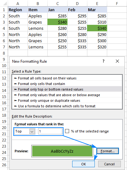
Microsoft Excel has a predefined rule to format top ranked values, which suits our needs perfectly. Here are the steps to apply it:
- Select your range of numbers (C2:C7 in our case).
- On the Home tab, in the Styles group, click Conditional formatting > New Rule.
- In the New Formatting Rule dialog box, choose Format only top or bottom ranked values.
- In the lower pane, pick Top from the drop-down list and type 1 in the box next to it (meaning you want to highlight just one cell containing the largest value).
- Click the Format button and select the desired format.
- Click OK twice to close both windows.
Done! The highest value in the selected range is automatically highlighted. If there is more than one max value (duplicates), Excel will highlight them all:
Highlight max value in each row
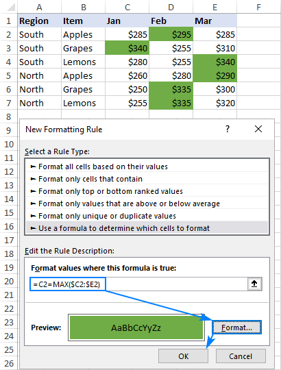
Since there is no built-in rule to make the highest value stand out from each row, you will have to configure your own one based on a MAX formula. Here's how:
- Select all the rows in which you want to highlight max values (C2:C7 in this example).
- On the Home tab, in the Styles group, click New Rule > Use a formula to determine which cells to format.
- In the Format values where this formula is true box, enter this formula:
=C2=MAX($C2:$E2)Where C2 is the leftmost cell and $C2:$E2 is the first row range. For the rule to work, be sure to lock the column coordinates in the range with the $ sign.
- Click the Format button and choose the format you want.
- Click OK twice.
Tip. In a similar manner, you can highlight the highest value in each column. The steps are exactly the same, except that you write a formula for the first column range and lock the row coordinates: =C2=MAX(C$2:C$7)
For more information, please see How to create a formula-based conditional formatting rule.
Excel MAX function not working
MAX is one of the most straightforward Excel functions to use. If against all expectations it does not work right, it's most likely to be one of the following issues.
MAX formula returns zero
If a normal MAX formula returns 0 even though there are higher numbers in the specified range, chances are those numbers are formatted as text. It's especially the case when you run the MAX function on data driven by other formulas. You can check this by using the ISNUMBER function, for example:
=ISNUMBER(A1)
If the above formula returns FALSE, the value in A1 is not numeric. Meaning, you should troubleshoot the original data, not a MAX formula.
MAX formula returns #N/A, #VALUE or other error
Please check the referenced cells carefully. If any of the referenced cells contains an error, a MAX formula will result in the same error. To bypass this, see how to get the max value ignoring all errors.
That's how to find max value in Excel. I thank you for reading and hope to see you on our blog soon!
 by
by
124 comments
Team Runs for the day Team Runs for the day Leading Team
South Vizag 7 Coimbatore 1 12 Coimbatore 1
Tirupathi 2 Erode 11 Erode
Hosur 10 Guntur 23 Guntur
Nellore 10 Madurai 1 12 Madurai 1
Salem 8 Strategic Br-Hyderabad Main 3 Salem
In this above i have to compare two teams and should reflect highest team name?? how please suggest ???
Please clarify your specific problem or provide additional details to highlight exactly what you need. As it's currently written, it's hard to tell exactly what you're asking.
Hi,
Product SKU Current Location Age
FNSF51LGRU30003 47
FNSF51LGRU30003 46
FNSF51LGRU30003 46
If i use the max if formula for the above data. The data is identifying the high value number in it for all the same SKU.
I need to freeze it if once the answer used.
For Example : 47 should occur only once. Next answer for the FNSF51LGRU30003 should be 46. Not the same 47.
Plz help me out.
Hi!
Based on your description, it is hard to completely understand your task. However, I’ll try to guess and offer you MAXIFS formula
=MAXIFS(B1:B3,A1:A3,"FNSF51LGRU30003")
if three different numbers , make 2 sets of pair, find the minimum difference in that 2 sets of pair that should less than 15 and how to finalize the highest values minimum difference pair.
Hi!
To find the minimum difference, use the MIN function.
Article Material Desc BUn CC Code Base Rate
590000002 APPLE RED DELICIOUS (KG) KG AV53 145
590000003 APPLE GRANNY SMITH (KG) KG AM43 169.8
590000005 APPLE ROYAL GALA (KG) KG AV53 150
590000008 APPLE KINNOR (KG) KG AM42 126.4
590000008 APPLE KINNOR (KG) KG AM43 134
590000017 AVACADO (KG) KG AV53 240
590000024 PASSION FRUIT KG AV53 110
590000034 GRAPES IMPORTED (KG) KG AM42 366.3
590000036 GRAPES BANGALORE BLUE KG AK75 45
590000039 GRAPES FLAME SEEDLESS KG S577 77
590000042 GRAPES SONAKA SEEDLESS KG AK51 50.5
590000042 GRAPES SONAKA SEEDLESS KG AK74 51
590000042 GRAPES SONAKA SEEDLESS KG VX53 54
590000047 MANGO TOTAPURI KG AK74 125
590000047 MANGO TOTAPURI KG AM43 158
590000047 MANGO TOTAPURI KG SKAC 110
590000051 MUSK MELON (KG) KG AK74 20
590000051 MUSK MELON (KG) KG AM43 24.7
590000051 MUSK MELON (KG) KG SB81 22
How to highlight, each max value in E column, against data in A or B column
eg. For musk melon max value is 24.7, so only it has to highlighted..like that to do for each products
It would be of great help if I get solution for this
Hello!
To find the maximum value by condition, use the MAXIFS function. I recommend reading this article: MAXIFS function in Excel – find max value with multiple criteria.
For example,
=MAXIFS(E2:E20,B2:B20, "MUSK MELON")
I need to find the top 5 highest values from this set of data:
64.47
59.2
58.77
55.94
75.54
63.01
57.65
54.91
54.01
58.94
51.33
55.86
71.09
53.69
72.33
59.05
66.53
53.95
what formula should I use?
Hello!
The answer to your question can be found in this article: Excel LARGE function with formula examples to get n-th highest value.
Thanks, So helpful!!!
I have a data on Matrix and I also have the criteria data in Matrix as well See below
Data from the Matrix
Period 0.0 30 45 60 75 90 105 120 135 150 180
6.0 0.356 0.443 0.469 0.505 0.579 0.525 0.516 0.475 0.342 0.271 0.171
7.0 0.439 0.541 0.558 0.678 0.802 0.642 0.747 0.499 0.436 0.336 0.232
8.0 0.505 0.544 0.591 0.694 0.759 0.747 0.736 0.584 0.560 0.467 0.269
9.0 0.489 0.614 0.618 0.630 0.791 0.687 0.631 0.577 0.507 0.562 0.340
10.0 0.538 0.603 0.572 0.580 0.703 0.643 0.619 0.556 0.489 0.459 0.399
11.0 0.503 0.491 0.513 0.578 0.585 0.630 0.587 0.542 0.439 0.459 0.345
12.0 0.517 0.446 0.539 0.588 0.546 0.564 0.552 0.497 0.411 0.412 0.355
13.0 0.470 0.439 0.545 0.534 0.530 0.482 0.510 0.470 0.422 0.404 0.329
14.0 0.399 0.427 0.469 0.442 0.462 0.434 0.409 0.425 0.382 0.395 0.340
15.0 0.370 0.390 0.388 0.397 0.421 0.393 0.355 0.387 0.355 0.341 0.331
Criteria for the matrix
Period 0.0 30 45 60 75 90 105 120 135 150 180
6.0 3 5 5 6 7 6 6 5 3 2 0
7.0 5 6 7 9 10 8 10 6 5 3 1
8.0 6 6 7 9 10 10 9 7 7 5 2
9.0 6 8 8 8 10 9 8 7 6 7 3
10.0 6 7 7 7 9 8 8 7 6 5 4
11.0 6 6 6 7 7 8 7 6 5 5 3
12.0 6 5 6 7 6 7 7 6 4 4 3
13.0 5 5 6 6 6 5 6 5 4 4 3
14.0 4 5 5 5 5 5 4 5 4 4 3
15.0 4 4 4 4 4 4 3 4 3 3 3
Is there any way to find the maximum of no 3 or 10 from the criteria data on the criteria Matrix, and the max values should be taken the matrix data based on the location from the matrix criteria ?
So from the above No 10 should be the maximum from Matrix ( [7,75] or [7,105] or [8,75] or [8,90] or [9,75] )?
Thanks for your help and taughts
I like it
I need to get the list of highest defect type from the product type of highest defect contributor with list of data below.
Process Type Total NG Input Output Defect 1 Defect 2 Defect 3 Defect 4 Defect 5
A AA 10 20 10 5 5 0 0 0
A AC 15 20 5 0 7 8 0 0
A AD 12 20 8 0 6 2 4 0
A AB 10 20 10 3 3 4 0 0
A AD 10 20 10 0 5 5 0 0
A AG 10 20 10 0 0 5 5 0
B AF 16 20 4 0 10 3 3 0
B AC 13 20 7 0 0 6 7 0
B AR 10 20 10 0 0 4 6 0
B AD 10 20 10 0 0 0 5 5
B AB 10 20 10 0 0 0 5 5
B AR 10 20 10 0 0 5 5 0
C AJ 12 20 9 0 0 6 6 0
C AS 10 20 10 5 5 0 0 0
C AF 10 20 10 0 5 5 0 0
C AA 10 20 10 0 0 0 5 5
Where Output data should be like this
Process Type Total NG Input Output Highest Defect Quantity Highest Defect Type
A AC 15 20 5 7 Defect 2
B AF 16 20 4 10 Defect 2
C AJ 12 20 9 6 Defect 3
C AJ 12 20 9 6 Defect 4
Thank you for the response
Hi!
I don't really understand how you want to create a list. For example, why is it missing B AC 13 20 7 0 0 6 7 0. I don't think it's possible to do this with a single formula. Perhaps this guide will be helpful: How to get matches of largest N values.
If you have a specific question about the operation of a function or formula, I will try to answer it.
I scourged the net and found this helpful, but ran into a dead end. I have a spreadsheet that has incidents in other.
Sheet/tab #1: Overview tab of all collected incidents, with the latest comment copied/paste from the other tabs.
A2: Incident #, B2: Date Reported, C2: Status, D2: Latest Comment
Sheet #2: has information on the all the information on this incident 2 by date (A2:A100) including latest comments all in column D.
A2: Date, B2: Assignee, C2: Updated by, D2: Comment
Sheet #3: same as #2
...etc...
Each sheet is named the Incident Number. So for example, incident "#2" is also the same name of the reference sheet "#2".
As the incidents are growing, I need to automate this to pull the max date's "Comment" from each sheet directly to the overview sheet #1 corresponding to that incident # in each row (D2). Currently I'm manually updating D2 Comment cell's formula's sheet reference:
=VLOOKUP(MAX('#2'!$A$2:$A$100),'#2'!$A$2:$D$100,4,0)
which is becoming tedious. Is there a way to automate pulling from the sheets (e.g. #2, #3, etc.) other than manually naming the sheet reference in the formula? I tried to concatenate '#2' to pull from A2 but that didn't work.
Any help is greatly appreciated!
Hello!
To create a dynamic reference, use the INDIRECT function. For example,
=INDIRECT("'"&A2&"'!A2:A100")
where A2 = "#2".
For more information, please visit: Excel INDIRECT function - basic uses and formula examples
You probably already know this, BUT you're a genius! Got it working!**
I guess I was just off by missing a few small things. In case anyone else needs it:
=VLOOKUP(MAX(INDIRECT("'"&A2&"'!A2:A100")),INDIRECT("'"&A2&"'!A2:D100"),4,0)
Again, you guys are awesome!!!
TLDR:
**this works off my master list that pulls my comments (in column 4) from other sheets. The master references list is written in cell A2 (with the sheets/tab being the same name), and then looks at the max date in cell A2:A100, from the table A2:D100, pulling back the latest comment listed in column 4.
I have a spreadsheet to hold a series of quiz results
Quiz Number of questions Contestant 1 Score Fractional score Max Score
1 40 25.5 0.6375 18
2 30 17 0.566666667
3 20 18 0.9
I want a formula that calculates the "Max Score", based on the highest "Fractional Score". To calculate "Fractional Score" I divide the actual score by the number of questions.
I can calculate "Max Score" using
=INDIRECT("C"&MATCH(MAX($D:$D),($D:$D),0))
In the sample the "Max Score" is 18 ie the value in Column C where the highest value of "Fractional Score" occurs.
I want to do this without showing or using the "Fractional Score" column. I have tried such things as:
=INDIRECT("C"&MATCH(MAX($C:$C/$B:$B),$C:$C/$B:$B,0))
but it shows #N/A.
Would you be able to help?
Hello!
If I understood you correctly, then you can use INDEX MATCH to find Max Score.
=INDEX(E1:E3,MATCH(MAX(C1:C3/B1:B3),C1:C3/B1:B3,0))
Hope this is what you need.
Hi,
Thanks for that! I needed to replace "E1:E3" with "C1:C3" and enter it using SHIFT/CTRL/RTN, but it works perfectly. I now need to figure out how I can use whole column references (eg "C:C" rather than "C1:C3") so that I don't have to edit it every time a new row is added.
Thanks again.
I have a data table with datewise sales. each date has lot of number of transactions. I want to find a date and value of sales with highest value (Highest value of sales in a day)
Hi!
The following tutorial should help to find the maximum value for a specific date: Excel MAX IF formula to find largest value with conditions.
I'm trying to calculate my students' grades. They take 4 exams. The highest (max) is weighted a bit more than the other 3. So, I'd like to create a function to identify the max of the 4 #s, multiply it by .2, and then take the other 3 #s and multiply each by .15, and then add them all together. I appreciate your help!
Hi!
If I understood you correctly, determine the maximum value using the MAX function and subtract it from the total grades.
=MAX(A1:A4)*0.2+(SUM(A1:A4)-MAX(A1:A4))*0.15
Hello Everyone,
How to automatically find the amount using the cut-off date?
just so happened no dates for 01/31/2021, instead, the date before that could be taken
Result must be 700.00
Cut-off Date: 01/31/2021
Amount: ?
Date Amount
12/31/2020 1,000.00
12/31/2020 700.00 (this must be the result)
02/28/2021 900.00
04/14/2021 800.00
04/30/2021 1,200.00
05/14/2021 500.00
06/30/2021 600.00
I cannot find the right formula, pls help me do it correctly.
thank you very much.
Hi!
Use VLOOKUP function with approximate match:
=VLOOKUP(DATEVALUE("01/31/2021"),A1:B7,2,TRUE)
I hope my advice will help you solve your task.
I have cell address written in text. Would like to know how to find the max value from the defined addresses.
Example:
Cell A1 input text as $C$56
Cell A2 input text as $C$12356
Would like to find max($C$56:$C$12356)
Instead of selecting the cell range manually, the formula should success based on the text input in A1 & A2.
Hello!
Use the INDIRECT function to convert text into a cell address. See formula examples here: How to use INDIRECT function in Excel.
The formula below will do the trick for you:
=MAX(INDIRECT(A1&":"&A2))
got the solution. Using indirect().
Max(indirect(A1):indirect(A2))
Hello!
In one of the data's column (let's say it's "A") I have DATE information (formatted like this: 03/14/01) and in the other column (let's say "B") I have PERCENTAGE value that changes based on some other data. Now, what I'd like to obtain is to have a MAXIMUM value of the PERCENTAGE column based on any given MONTH (January, February, March and so on). For example: what is the maximum percentage value for a month of January or February or March, etc..?
Can someone please help me with a formula here?
Thank you,
Julia
Hello!
You can get max value within a date range using the MAXIFS function. Look for the example formulas here: MAXIFS function - get largest value based on multiple criteria.
Hi,
I am trying to return the Highest value from the below row considering the condition if A>B>C>D. The formula should return the highest value meeting the condition.
A Approved
B Approved with Comments
C Resubmit
D Rejected
A>B>C>D
D D C C C B B B A A "=FORMULA"
Hello!
If your values are written in separate cells, then you can extract the desired letter using the INDEX + MATCH formula:
=INDEX(B2:K2,MATCH(MIN( MATCH(B2:K2,{"A","B","C","D","E","F","G","H","I","K","L","M", "N","O","P","Q","R","S","T","U","V","X","Y","Z"},0)), MATCH(B2:K2,{"A","B","C","D","E","F","G","H","I","K","L","M", "N","O","P","Q","R","S","T","U","V","X","Y","Z"},0),0))
Hi,
I got the solution by below formula:-
=IFERROR(CHAR(MIN(CODE("A"),CODE("B"),CODE("C"),CODE("D")),"")
Thanks for your help .
RANDUM NUMBER ENTRY STOCK PICK THIS RESULT
65.500 12.5+12.5+24.5+30+70+65.5 12.5+12.5+24.5+30
I have a spreadsheet that calculates used/monthly accrued vacation time based on hours and minutes.
Example: Hours/Minutes total for May shows 150:10 (the formula used to arrive at this figure is =SUM(F6-B7+E7). I need to add or edit this formula to tell it to max out and never exceed an accrual of more than 283:30. I tried =MAX(F36-B37+E37,&TIME(“283:30,0,0”), but that was not successful. Do you have any suggestions?
Hello!
With the TIME function, you cannot set the time for more than 24 hours. Convert your time to days with this formula
=283.5/24
If I understand your task correctly, use MIN function and try the following formula:
=MIN(F36-B37+E37,283.5/24)
That worked! Thank you.
Can I use the MAX formula on a cell range that uses IF formula's to display a number?
Ex.
2 Mild ("2" is displayed using [=IF('Severity Rating'.I3="Yes";"2";"0")])
3 Moderate ("3" is displayed using [=IF('Severity Rating'.I4="Yes";"3";"0")])
4 Severe ("4" is displayed using [=IF('Severity Rating'.I5="Yes";"4";"0")])
I want to create a function to identify the max number (4 in this case) and sum all the severity ratings in each category (the above is just one category). The IF formula identifies if Mild, Moderate, or Severe ratings were indicated by the client, but I don't want to add all of them, as that would be inaccurate. There are 5 separate categories with 20 being the highest score possible. I only want to sum the highest number displayed in each category.
Hope that makes sense! Thanks for any help you can offer!
- Catinreno
Hello!
To find the largest number in each category, use the MAXIFS function.
Except apparently that won't work in open office Calc. Any other options?
Hi!
I can't give you any advice about Open Office, sorry. This is a blog about Microsoft Office.
In Excel, what would the formula for this look like? From what I am understanding, the Max_range & Criteria_range1 are identical?? And then what would be the criteria1?
Here's the list again for reference (It looks like I might have accidentally deleted the first row in my first post):
1 Absent ("0" or "1" is displayed using [=IF((AND('Severity Rating'.I3="No",'Severity Rating'.I4="No",'Severity Rating'.I15="No")),"1","0")])
2 Mild ("2" is displayed using [=IF('Severity Rating'.I3="Yes";"2";"0")])
3 Moderate ("3" is displayed using [=IF('Severity Rating'.I4="Yes";"3";"0")])
4 Severe ("4" is displayed using [=IF('Severity Rating'.I5="Yes";"4";"0")])
Thanks again.
Heya! I'm trying to create a football playoff scores tracker/spreadhseet, and I want to answer the following question: 'Out of this column of scores, what is the highest score?' Except, I need it to return the team name (adjacent to the cell containing their score), not just the highest number. I grasp how to use the max function for this, just not sure how to extend it to return a different field.
Thanks!
Hi!
Use the FILTER function to return the row with the maximum value in the column.
Use the formula like this:
=FILTER(A2:B9,B2:B9=MAX(B2:B9))
Can you please be more specific on this. where to use that formula?
I have a sheet to record performance. So names, in column A, then figures for each day of the week in B to F. I've got the highest values for each row selected in column L, but now i Struggle to sort them in order, so names and the highest values respectively, in highest to lowest order?
Hello!
If I understand correctly, you want to get columns A and L and sort them. Please use the formula below:
=SORT(FILTER(A1:L8,(COLUMN(A1:L8)=1) + (COLUMN(A1:L8)=12)),2,-1,FALSE)
You can learn more about FILTER function in Excel in this article on our blog.
Also take a look at this article: SORT function - automatically sort with formula.
Hi, I am trying to find the max value in cells containing letters in the beginning and numbers aftewards. i.e AB22002, CC22021, CB22003. Can I get the max of the numbers only. I am trying to avoid to have to split them in different cells.
Thanks,
Tony
Hi!
Your cells contain text, so you need to extract numbers from the text. For example, using the MID function extract all characters starting from the third and convert text to numbers:
=MAX(--MID(A2:A30,3,20))
This should solve your task.
Hello! How to find the highest number using the IF condition?
Hi!
Why can't you use the MAX function to find the maximum value?
Hello,
I would like to count the the latest date in each row (spanning columns B through F) that are equal to or less than another date in a separate row (Column A). I though maybe the Max feature might be helpful. Am a bit frustrated. What I am trying to do is retroactively count (based on a specific date in Column A) the number of students that had attained various levels of academic achievement (signified by Levels 3,4,5 etc) by that date is Column A.
Hello!
To conditionally count, use the COUNTIF or COUNTIFS function. You can find examples and detailed instructions in this article. I hope I answered your question. If this is not what you wanted, please describe the problem in more detail.
how to find a maximum items?
like in your example here I want to get the highest cost fruit if it is grapes,lemon, apple
I want a function that writes a word (which is items in your example) not a number.
thank you!
Hello!
To select the product with the maximum price from the list, use the INDEX+MATCH functions
=INDEX(B3:B8,MATCH(TRUE,$C$3:$C$8=MAX($C$3:$C$8),0))
I hope I answered your question. If something is still unclear, please feel free to ask.
im trying to find the best way to write a function that will take the max of a range of cells and display the row header associated with that cell... for example take the Max of cells A1:a17 and display the row header of whichever value is produced from the max function. any input?
Hi!
Your question is not entirely clear. What row title do you want to show? What cells is the row header in?
Is it possible to do an index match lookup between 2 tables and also find the highest value? The index match + max formulas I am finding all seem to be for within a single table.
For example, if you have a list of cities and hotel prices at different times of the year in one table.
Then in another table, you have a list of cities, with columns for different values and you want to pull in the highest hotel price from the other table. Is that possible with any kind of lookup?
Hello!
I recommend reading this guide: VLOOKUP across multiple sheets in Excel with examples.
I hope my advice will help you solve your task.
Hello,
I have tried my best on my own forever. I am trying to get the largest sum of 5 numbers, however, based on a second column, the corresponding total cannot exceed a number. Example, for the below, I would like to have the left column total the largest of the 5 added up, but cannot exceed $135 based on the column to it's right. I have gotten close, but it will give me a number but don't actually know which 5 it has chosen! Ha. So best case scenario, it will highlight or say A, D, H or whatever are the five that total the most without going over $135 summed on the right column. Thanks for any help and I hope that makes sense.
A 24.91 $37
B 19.47 $23
C 18.26 $38
So On 17.27 $34
13.48 $22
12.37 $18
11.45 $20
10.68 $18
9.49 $17
9.34 $18
8.99 $16
6.25 $10
6.15 $21
5.38 $10
4.28 $10
I have a customer list with three columns representing stage1, stage2 and stage3. some customers have balance only in one stage while others have balance in two stages. I want to find out the stage with maximum balance for each customer. how to find the same.
Customer STAGE1 STAGE2 STAGE3 Result I want
ABC 100 400 STAGE3
DEF 3000 2000 STAGE1
MNO 5000 50 STAGE2
KPL 250 STAGE1
GHI -250 STAGE2
How can I find the result with a formula for larger amount of data
Hello!
The formula below will do the trick for you:
=INDEX($B$1:$D$1,MATCH(MAX(B2:D2),B2:D2,0))
You can learn more about searching with INDEX + MATCH in Excel in this article on our blog.
I have 2 columns of values, i have conditionally formatted each to show top 20%. I want ones that are in the top 20% of each category to be highlighted in another colour. e.g top 20% in column A Green, top 20% in column B Green. In top 20% in A and B Blue.
Any assistance is appreciated
Thanks,
Luke
Hello!
Here is the article that may be helpful to you: How to change background color in Excel based on cell value.
After I find the MAX value, do I use a CONCATENATE formula to show which is the highest value? Any suggestions are welcome. Thank you.
Hello!
You can insert the maximum value returned by the MAX function into a text string using the CONCATENATE function:
=CONCATENATE("Maximum value ",MAX(A2:A20))
i have in
column A: 34,34,34,33,33,33,35,35.
column B: 3,2,1,5,4,3,2,2,1
what function i can use to gate max value of B compare to A: 34,33,35 for each
like in column C: 3,nil,nil,5,nil,nil,2,nil.
Hello!
Use the MAXIFS function:
=IF(B2<>MAXIFS($B$2:$B$9,$A$2:$A$9,A2),0,MAXIFS($B$2:$B$9,$A$2:$A$9,A2))
This should solve your task.
I have been trying the formula to get headers to find maximum value in rows which goes as =INDEX($P1:$R1,0,MATCH(MAX($P2:$R2),$P2:$R2,0))
I drag the formula through the column. It takes the 2nd row values as headers. The formula seems as =INDEX($P2:$R2,0,MATCH(MAX($P3:$R3),$P3:$R3,0)). It returns the 2nd row maximum values in the consecutive cells but not headers for the maximum value.
How can I fix this issue that the header reference formulas do not change in the formula?
Hello im trying to find the best formula for this data. I feel it should be FILTER but not sure which one to use.
I need to filter the result in column D with the condition as
amount = highest value in Column C
data limited to column B of Company XYZ
expected result should be: A9100 amount$3,428.52
please help.. I'm not expert in excel's formula. thanks in advance..!!
A B C D
Company XYZ AC1000000454 $3.59 A1019
Company XYZ AC1000000454 $67.91 AR400
Company XYZ AC1000000454 $3,428.52 A9100
Company XYZ AC1000000454 ($353.20) AF400
Company XYZ AC1000000454 ($33.00) AHF00
Company XYZ AC1000000454 ($4,256.00) A1044
Hi,
Could you please help me out on how to calculate max time from an array of 3 time stamps of 3 systems placed horizontal in range? How can I get the system names too after I try the formula or it can directly show system names that has highest time? How can I use maxifs with criteria range?
System 1, 00:30:23
System 2, 00:57:20
System 3, 00:11:05
Hello!
If I understand your task correctly, the following formula should work for you:
=INDEX(A1:A10,MATCH(MAX(B1:B10),B1:B10,0))
Hi,
The 3 time stamps are placed horizontal on a row.
A. B. C
00:30:23. 00:57:20 00:11:05
How can I get max value from the columns A,B,C with names system 1, system2 and systems 3 respectively in formula? Please help me out on this.
Hi!
Have you tried the ways described in this blog post? If they don’t work for you, write what formula you used and what were the problems.
Hi,
I have tried with index, match, max functions.
If I have headers : System1, System2, System3 in Column O, P, Q with 00:01:57, 00:04:00, 00:00:35 timestamps respectively.
And there is a list of 50 timestamps under each.
I want to find out which system has maximum timestamp value.
I tried the formula, on 2nd row:
INDEX($O1:$Q1,0,MATCH(MAX($O2:$Q2),$O2:$Q2,0))
Problem1 : I don’t get the true system header name with true maximum value.
Problem 2: the formula doesn’t work on 3rd row when I try to drag the formula for next 50 rows.
Please suggest.
Hello!
If I got you right, the formula below will help you with your task:
=INDIRECT(ADDRESS(1,MIN(IF(O2:Q51=MAX(O2:Q51),COLUMN(O1:Q1)))))
This is an array formula and it needs to be entered via Ctrl + Shift + Enter, not just Enter.
I hope it’ll be helpful.
How can I get any of the three systems names whichever with maximum value on a single column with respect to 50 rows for 3 systems?
Hi
Am working with data where I have to get the date of Highest Quantity with matching Product No.
Maxif formula is not working with.
Kindly suggest the way out.
Product Qty Date
GHI 102 30-Aug
DEF 77 30-Aug
ABC 21 30-Aug
ABC 10 30-Aug
GHI 119 20-May
GHI 106 20-May
GHI 94 20-May
DEF 81 20-May
DEF 69 20-May
DEF 56 20-May
ABC 44 20-May
ABC 36 20-May
ABC 10 20-May
GHI 114 10-May
DEF 90 10-May
DEF 65 10-May
ABC 40 10-May
ABC 20 10-May
GHI 110 01-May
DEF 85 01-May
DEF 61 01-May
ABC 35 01-May
GHI 123 30-Apr
GHI 98 10-Apr
DEF 73 10-Apr
ABC 48 10-Apr
ABC 30 10-Apr
Result should be - ABC - 10-Apr (ABC highest Qty is 48 so 10-Apr)
Hello!
Specify which formula you are using. Also, check if your date is written as text.
Hi
Date format is correct.
Have tried {=MAX(IF($B$3:$B$29=$G6,$D$3:$D$29))}
This gives me latest date against ABC which is 30-Aug.
I would like to have result 10-Apr because ABC has 48 (highest Value)
Hello!
I believe the following formula will help you solve your task:
=FILTER($D$3:$D$29,($B$3:$B$29=$G$6)*($C$3:$C$29=MAXIFS($C$3:$C$29,$B$3:$B$29,$G$6)))
You can learn more about FILTER function in Excel in this article on our blog.
Hello,
Does anyone know how to apply this function with data that is not in a consecutive range?
Instead of a range like B5:G5, my data is B5,D5,F5,
Can anyone help?
Thanks!
Hi!
You can use this formula:
=MAX(B5,D5,F5)
Hi,
I have a data sheet that I need to extract information from, in one column I have the NAMES of persons, in another I have either "yes" or "no" answers for each person.
I'd like to extract everyone's name who answered "yes" into either one cell, separated by commas, or each into a vertical list.
Hello!
I recommend reading this guide: Excel FILTER function - dynamic filtering with formulas.
I hope I answered your question. If something is still unclear, please feel free to ask.
Hi, I am involved in stock trading and i have my trading records in Excel; ie bunch of profits and losses.
My question is, how do i find the lowest and highest profit and loss that i make in my records?
=MAX(IFERROR(P23:P79, "")) + CTRL + Shift + Enter only return highest profit, while
=MIN(IFERROR(P23:P79, "")) + CTRL + Shift + Enter returns highest loss.
How do i find lowest profit and lowest loss? Where can i fit the criteria "0" ?
Do note that i have multiple blanks (intentionally left) and #DIV/0! (formula i keyed in in advance for future trading but i havent filled in respective fields)
Thank you in advance. God bless and have a nice day.
Hello!
To find the lowest loss, use the formula
=MAXIFS(A1:A10,A1:A10," < 0")
Minimum profit -
=MINIFS(A1:A10,A1:A10," > 0")
Please have a look at this article: MINIFS function in Microsoft Excel and MAXIFS function in Excel.
Hello, I'm trying to get the maximum error to show up but some times the maximum error is a negative (so -5 is a greater error than +3 etc) Any ideas?
Also the 2 cells I'm comparing arent next to each other (just to add to the fun).
hello
Can I get help to write a formula that will highlight the lowest price for an article that repeats in several rows. If that article only shows once then that price would be highlighted too. for example only the first line would be highlighted.
article 1 300
article 1 548
article 1 2500
Thank you for your help
Hello!
I recommend using the FILTER function to find the article you are looking for. Find the minimum price using the MAXIFS function.
=FILTER(A1:B8,(A1:A8="article 1")*(B1:B8=MINIFS(B1:B8,A1:A8,A1:A8)))
I hope my advice will help you solve your task.
I'm struggling with this a bit.
My challenge is that I've got a list of results in a column, and want to identify the largest value in that column and then add a bonus prize in the next column for the largest row value.
I would describe it BADLY as:
in the column next to the data: +IF("the data in this cell is greater than the cells in rh column, give me A point" otherwise 0)
Does that make sense?
thanks
Hello!
In the next column, you can write the formula
=IF(MAX($A$1:$A$30)=A1,100,"")
After that you can copy this formula down along the column.
Hope this is what you need.
I am trying to find a formula that returns for example to find which State had the highest sales for a specific month. Column A is the State and Column B is the sales for the specific month. Does anyone know a formula for this? Thanks.
Hello!
The formula below will do the trick for you:
=INDEX(A1:A50,MATCH(MAX(B1:B50),B1:B50,0))
Here is the article that may be helpful to you: INDEX function in Excel
Thanks it worked.
Well if my range is - A2:D10 and I need to find the highest value with the name the person
Hi, is it possible to create a formula to find the max value if some of the cells contain ranges please?
i.e. working out that the max value is 505 from the following cells:
Cell 1. 490
Cell 2. 500,
Cell 3. 490-505
Dear Sir
can you help me to do a formula to find highest value of 1st numbers letters
This is excellent, thanks for saving me a ton of time!
which one of the following functions is designed to display the maximum value in a range of cells with question answer
THANK YOU!!! Do you know how complicated I have been making this for years?! And it was as simple as =Max!!!
You have made my day!
How to find max, 2nd, 3rd & 4th latest dates by name in another sheet?
Results e;
Names in column A
Dates in column B
Distance in column C
& so on
Regards
Tony
Well nd easy