Trying to get a bottom value based on one or more conditions? Just use the SMALL function together with IF. This tutorial shows how to build a working solution and explains its internal logic, so that you could easily decipher the formula and adjust for your needs.
Microsoft Excel has a number of functions to do "conditional" calculations such as MAXIFS, MINIFS, AVERAGEIF, and the like. Regrettably, the SMALL IF function does not exist. However, nothing prevents you from building your own formula to find the n-th smallest value with criteria. If you are not familiar with the Excel SMALL function yet, then you might want to start with the basics and read the above linked tutorial first.
SMALL IF formula in Excel
To get the n-th lowest value that matches the criteria you specify, you can use the following generic formula:
Where n is the 1st, 2nd, 3rd, etc. lowest value to return.
For the formula to work correctly, you should enter it as an array formula by pressing the Ctrl + Shift + Enter keys simultaneously. When you do this, Excel will surround the formula in curly brackets like shown in the screenshot below. In Excel 365, it also works as a regular formula due to support for dynamic arrays.
From our sample the table, let's pick bottom 3 scores in a specific subject, say Art. With the list of subjects (criteria_range) in B2:B15, scores in C2:C15 (values) and n in E3, the formula takes this form:
=SMALL(IF($B$2:$B$15="art", $C$2:$C$15), $E3)
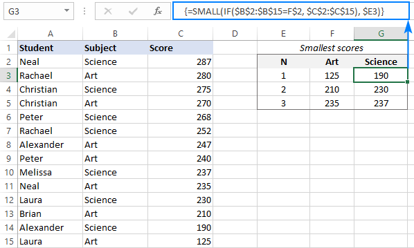
This formula returns the smallest Art score in F3. Copy it down through F5, and you will get the 2nd and 3rd lowest results.
For convenience, you can also input the names of the target subjects in predefined cells (F2 - Art and G2 - Science), and refer to those cells as criteria:
=SMALL(IF($B$2:$B$15=F$2, $C$2:$C$15), $E3)
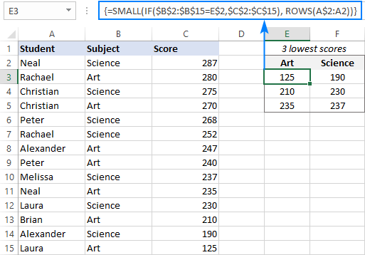
If the design of your worksheet does not provide for n numbers, you can generate them directly in the formula by using the ROWS function with an expanding range reference like this:
=SMALL(IF($B$2:$B$15=E$2,$C$2:$C$15), ROWS(A$2:A2))
Due to the clever use of absolute and relative references, the range reference expands automatically as the formula is copied to the below cells. In E3, ROWS(A$2:A2) generates n equal to 1, and the formula returns the smallest score for Art. In E4, the reference changes to A$2:A3 causing ROWS to return 2, so we get the 2nd smallest score, and so on.
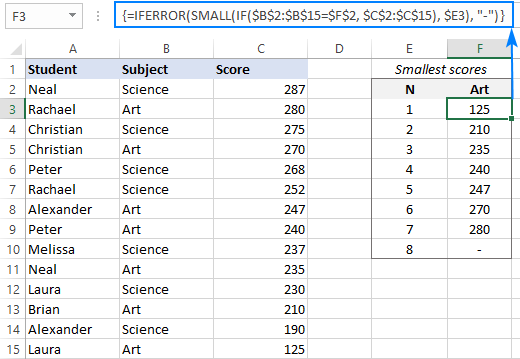
In case the n-th smallest value with specified criteria is not found, the SMALL IF formula would return a #NUM error. To trap this error and replace it with whatever value you find appropriate ("-" in our case), you can use the IFERROR function:
=IFERROR(SMALL(IF($B$2:$B$15=$F$2, $C$2:$C$15), $E3), "-")
How this formula works:
From an array supplied for the 1st argument, the SMALL function returns the n-th smallest value specified in the 2nd argument. The problem is that we do not want every single value in the array to be processed, but only the scores in a given subject. To limit the array to Art values, we tell the IF function to compare the list (B2:B15) against the target subject:
IF($B$2:$B$15="Art", $C$2:$C$15)
Because the logical test is performed on an array of numbers, the result is also an array, where the numbers represent the Art scores, and FALSE values any other scores:
{FALSE;280;FALSE;270;FALSE;FALSE;247;240;FALSE;235;FALSE;210;FALSE;125}
As the SMALL function ignores errors (and anything else that is not a number), the result is the n-th smallest value from the Art scores in the above array.
Excel SMALL IF with multiple criteria
To cause a SMALL IF formula to evaluate several conditions, choose one of the following approaches.
Supply multiple criteria by using nested IF statements:
Multiply the logical expressions:
Please notice that both are array formulas, so don't forget to press Ctrl + Shift + Enter to properly complete them. In Excel 365, these will also work as regular formulas.
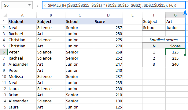
To test the formula "in the field", we will extend our sample table with the School column and input 2 criteria in separate cells like shown below.
Now, we have all needed parameters for our SMALL IF formula:
- Criteria_range1 - list of subjects (B2:B15)
- Criteria1 - target subject (G1)
- Criteria_range2 - school types (C2:C15)
- Criteria2 - target school (G2)
- Values - scores (D2:D15)
- N - numbers 1 to 3 in F6, F7 and F8
Putting the arguments together, we get these formulas:
=SMALL(IF($B$2:$B$15=$G$1, IF($C$2:$C$15=$G$2, $D$2:$D$15)), F6)
=SMALL(IF(($B$2:$B$15=$G$1) * ($C$2:$C$15=$G$2), $D$2:$D$15), F6)
Enter either one in G6, drag it through G8, and you will get the following result.
How these formulas work:
In essence, both formulas use the IF function to test multiple conditions, so that only the values for which all the conditions are TRUE get into the array argument of the SMALL function.
Nested IFs:
In the logical test of the first IF function, we compare the list of subjects against the target one (Art): $B$2:$B$15=$G$1. The result of this operation is an array of TRUE and FALSE values, where TRUE corresponds to the Art values in column B:
{FALSE;TRUE;FALSE;TRUE;FALSE;FALSE;TRUE;TRUE;FALSE;TRUE;FALSE;TRUE;FALSE;TRUE}
The second IF statement checks which cells in the range C2:C15 match the criterion in G2 (Junior), and also returns an array of TRUE and FALSE:
{FALSE;TRUE;TRUE;TRUE;FALSE;FALSE;TRUE;TRUE;FALSE;TRUE;TRUE;FALSE;FALSE;TRUE}
For the value_if_true argument of the second IF, we supply the scores (D2:D15). This ensures that only the items that have TRUE in the above two arrays "survive"; all other scores are replaced with the FALSE values:
{FALSE;280;FALSE;270;FALSE;FALSE;247;240;FALSE;235;FALSE;FALSE;FALSE;125}
This final array goes to the SMALL function, from which it returns the n-th lowest value.
Multiplying criteria:
The second formula checks both conditions within a single logical test, where the multiplication operation works as AND operator.
When the elements of two TRUE/FALSE arrays are multiplied, the logical values are converted to 1's (TRUE) and 0's (FALSE). As multiplying by 0 gives zero, the resulting array has 1 for data that meet both criteria:
{0;1;0;1;0;0;1;1;0;1;0;0;0;1}
The IF function evaluates this array of 1's and 0's in the logical test and passes the scores corresponding to 1's to SMALL.
SMALL IF formula with multiple OR criteria
The previous example shows how to find bottom values based on multiple criteria using AND logic, i.e. when all the conditions are satisfied. To get the smallest values that satisfy any of the conditions, you need to build a SMALL IF formula with OR logic. For this, add up the criteria instead of multiplying them.
As an example, let's pick the lowest scores in two different subjects, say History and Literature. In terms if Excel, the formula will return the n-th smallest score if Subject is either History OR Literature.
With the subjects in B2:B15 and scores in C2:C15, here's the formula to return the lowest score:
=SMALL(IF(($B$2:$B$15="History") + ($B$2:$B$15="Literature"), $C$2:$C$15), 1)
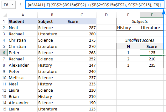
Of course, you can enter the criteria and n numbers in separate cells, complete the formula by pressing Ctrl + Shift + Enter and get this result:
=SMALL(IF(($B$2:$B$15=$E$2) + ($B$2:$B$15=$F$2), $C$2:$C$15), E6)
How this formula works:
The formula's logic is very similar to what is discussed in SMALL IF with multiple AND criteria example. The difference is that the range=criteria equations are joined with the addition operation that works like the OR operator in array formulas:
Checking the list of subjects against 2 different criteria yields 2 arrays of TRUE and FALSE values. Adding the elements of those arrays produces an array of 1's and 0's, where 1's correspond to the items that meet at least one condition (no matter which) and zeros correspond to the items that do not meet any condition. This final array goes to the logical test of IF:
{0;1;0;1;0;0;1;1;0;1;0;1;0;1}
The IF function evaluates each element of the above array and passes the scores corresponding to 1's to the SMALL function, from which it picks the specified n-th value:
{FALSE;280;FALSE;270;FALSE;FALSE;247;240;FALSE;235;FALSE;210;FALSE;125}
How to find smallest values ignoring zeros
Though your dataset may sometimes contain some zero values, it does not always make sense to include those zeros in the formula result. To leave out all 0 values, we will be using the already familiar SMALL IF formulas with the "not equal to zero" criteria.
Formula 1. SMALL IF not zero
To get the n-th smallest value ignoring 0, use this generic array formula:
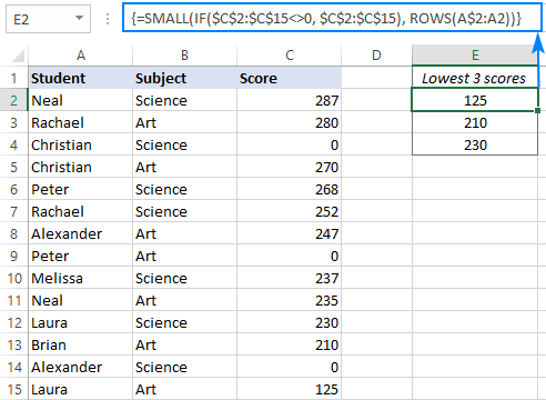
Suppose a few students missed some exams and have 0 scores for those subjects. To get the lowest 3 scores that are greater than 0, the formula is:
=SMALL(IF($C$2:$C$15<>0, $C$2:$C$15), ROWS(A$2:A2))
Please remember to press CTRL + Shift + Enter to complete it correctly.
This formula goes to the topmost cell (E2), into which it extracts the lowest score. And then, you drag the formula down through two more cells to extract the 2nd and 3rd lowest scores. The ROWS(A$2:A2) function automatically generates n numbers, so you needn't type them anywhere in the sheet.
Formula 2. SMALL IF greater than zero with condition
To find the n-th smallest value greater than zero based on criteria, place additional criteria in this way:
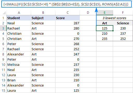
As an example, let's pull the bottom 3 scores for each subject individually. For this, we enter the subject names in E2 (Art) and F2 (Science) and use this formula to extract the smallest Art scores:
=SMALL(IF(($C$2:$C$15<>0) * ($B$2:$B$15=E$2), $C$2:$C$15), ROWS(A$2:A2))
Drag the formula to the right, and you will get the smallest Science scores too:
Filter smallest values based on criteria
This solution only works in recent builds of Excel 365 where dynamic array functions are available.
Another way to get the n-th bottom value in Excel based on conditions is using the SMALL function together with FILTER. This works beautifully as a normal formula completed with the Enter key.
The formula's logic is the same as in the previous examples. The difference is that you use the FILTER function instead of IF to apply the criteria.
Formula 1. Find n-th bottom value with one condition
If there is just one condition to be met, you can get the nth smallest value with this formula:
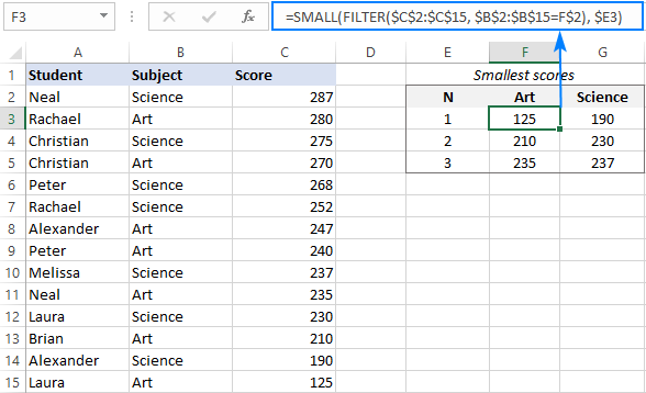
For our sample dataset, the formula goes as follows:
=SMALL(FILTER($C$2:$C$15, $B$2:$B$15=F$2), $E3)
Where B2:B15 is the criteria range (list of subjects), C2:C15 are the values (scores), F2 is the criteria (the subject of interest) and E3 is the n-th smallest score to return.
Formula 2. Get n-th smallest value with multiple criteria
To test multiple conditions, here's the formula to use:
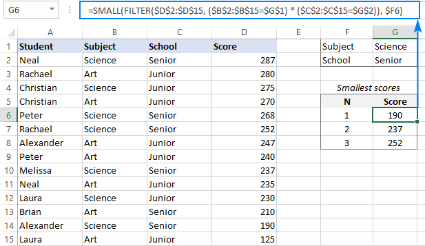
Assuming you are looking to find the n-th lowest score in a specific subject (G1) among students of a given school (G2), the formula is:
=SMALL(FILTER($D$2:$D$15, ($B$2:$B$15=$G$1) * ($C$2:$C$15=$G$2)), $F6)
Where B2:B15 is the list of subjects, C2:C15 are the school types, D2:D15 are the scores, and F6 is the n-th smallest value to return.
Formula 3. Filter n-th smallest value with OR criteria
To filter the n-th smallest number when this or that condition is TRUE, the formula is:
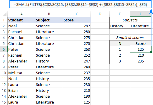
For instance, you can find the lowest score in humanitarian subjects (History or Literature) by using this formula:
=SMALL(FILTER($C$2:$C$15, ($B$2:$B$15=$E$2) + ($B$2:$B$15=$F$2)), $E6)
Where B2:B15 is the list of subjects, C2:C15 are the scores, E2 and F2 are the subjects of interest, and E6 is the n-th smallest value.
Tip. You can also use the SMALL function to extract bottom N records with advanced filter.
That's how to use SMALL IF in Excel to find smallest values based on conditions. I thank you for reading and hope to see you on our blog next week!
Practice workbook for download
Excel SMALL IF examples (.xlsx file)
 by
by
2 comments
Hi, thanks for the tutorial on small and if.
I am solving an issue of fixing a predefined value and then picking up the smallest number above that.
I am using a small & if function. However, i want to select the smallest value above a predefined value. E.g., looking at series of events and their timestamps however, want to pick the earliest after 5 AM.
I am using index formula with small + if
Thanks and regards.
Hi!
To find the nearest larger number you can try the formula
=INDEX(A2:A10,MATCH(MAX(IF((C1-A2:A10)>0,"",C1-A2:A10)),IF((C1-A2:A10)>0,"",C1-A2:A10),0))
С1 - predefined value
You can learn more about searching using INDEX+MATCH in Excel in this article on our blog.