 by
by The tutorial showcases a few different formulas to perform two dimensional lookup in Excel. Just look through the alternatives and choose your favorite :)
When searching for something in your Excel spreadsheets, most of the time you'd look up vertically in columns or horizontally in rows. But sometimes you need to look across both rows and columns. In other words, you aim to find a value at the intersection of a certain row and column. This is called matrix lookup (aka 2-dimensional or 2-way lookup), and this tutorial shows how to do it in 4 different ways.
Excel INDEX MATCH MATCH formula
The most popular way to do a two-way lookup in Excel is by using INDEX MATCH MATCH. This is a variation of the classic INDEX MATCH formula to which you add one more MATCH function in order to get both the row and column numbers:
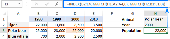
As an example, let's make a formula to pull a population of a certain animal in a given year from the table below. For starters, we define all the arguments:
- Data_array - B2:E4 (data cells, not including row and column headers)
- Vlookup_value - H1 (target animal)
- Lookup_column_range - A2:A4 (row headers: animal names) - A3:A4
- Hlookup_value - H2 (target year)
- Lookup_row_range - B1:E1 (column headers: years)
Put all the arguments together and you will get this formula for two-way lookup:
=INDEX(B2:E4, MATCH(H1, A2:A4, 0), MATCH(H2, B1:E1, 0))
If you need to do a two-way lookup with more than two criteria, take a look at this article: INDEX MATCH with multiple criteria in rows and columns.
How this formula works
While it may look a bit complex at first glance, the formula's logic is really straightforward and easy to understand. The INDEX function retrieves a value from the data array based on the row and column numbers, and two MATCH functions supply those numbers:
INDEX(B2:E4, row_num, column_num)
Here, we leverage the ability of MATCH(lookup_value, lookup_array, [match_type]) to return a relative position of lookup_value in lookup_array.
So, to get the row number, we search for the animal of interest (H1) across the row headers (A2:A4):
MATCH(H1, A2:A4, 0)
To get the column number, we search for the target year (H2) across the column headers (B1:E1):
MATCH(H2, B1:E1, 0)
In both cases, we look for exact match by setting the 3rd argument to 0.
In this example, the first MATCH returns 2 because our vlookup value (Polar bear) is found in A3, which is the 2nd cell in A2:A4. The second MATCH returns 3 because the hlookup value (2000) is found in D1, which is the 3rd cell in B1:E1.
Given the above, the formula reduces to:
INDEX(B2:E4, 2, 3)
And return a value at the intersection of the 2nd row and 3rd column in the data array B2:E4, which is a value in the cell D3.
VLOOKUP and MATCH formula for 2-way lookup
Another way to do a two-dimensional lookup in Excel is by using a combination of VLOOKUP and MATCH functions:
For our sample table, the formula takes the following shape:
=VLOOKUP(H1, A2:E4, MATCH(H2, A1:E1, 0), FALSE)
Where:
- Table_array - A2:E4 (data cells including row headers)
- Vlookup_value - H1 (target animal)
- Hlookup_value - H2 (target year)
- Lookup_row_range - A1:E1 (column headers: years)

How this formula works
The core of the formula is the VLOOKUP function configured for exact match (the last argument set to FALSE), which searches for the lookup value (H1) in the first column of the table array (A2:E4) and returns a value from another column in the same row. To determine which column to return a value from, you use the MATCH function that is also configured for exact match (the last argument set to 0):
MATCH(H2, A1:E1, 0)
MATCH searches for the value in H2 across the column headers (A1:E1) and returns the relative position of the found cell. In our case, the target year (2010) is found in E1, which is 5th in the lookup array. So, the number 5 goes to the col_index_num argument of VLOOKUP:
VLOOKUP(H1, A2:E4, 5, FALSE)
VLOOKUP takes it from there, finds an exact match for its lookup value in A2 and returns a value from the 5th column in the same row, which is the cell E2.
Important note! For the formula to work correctly, table_array (A2:E4) of VLOOKUP and lookup_array of MATCH (A1:E1) must have the same number of columns, otherwise the number passed by MATCH to col_index_num will be incorrect (won't correspond to the column's position in table_array).
XLOOKUP function to look in rows and columns
Recently Microsoft has introduced one more function in Excel that is meant to replace all existing lookup functions such as VLOOKUP, HLOOKUP and INDEX MATCH. Among other things, XLOOKUP can look at the intersection of a specific row and column:
For our sample data set, the formula goes as follows:
=XLOOKUP(H1, A2:A4, XLOOKUP(H2, B1:E1, B2:E4))

Note. The XLOOKUP function is only available in Excel for Microsoft 365, Excel 2021, and Excel for the web.
How this formula works
The formula uses the ability of XLOOKUP to return an entire row or column. The inner function searches for the target year in the header row and returns all the values for that year (in this example, for year 1980). Those values go to the return_array argument of the outer XLOOKUP:
XLOOKUP(H1, A2:A4, {22000;25000;700}))
The outer XLOOKUP function searches for the target animal across the column headers and returns the value in the same position from the return_array.
SUMPRODUCT formula for two-way lookup
The SUMPRODUCT function is like a Swiss knife in Excel – it can do so many things beyond its designated purpose, especially when it comes to evaluating multiple criteria.
To look up two criteria, in rows and columns, use this generic formula:
To perform a 2-way lookup in our dataset, the formula goes as follows:
=SUMPRODUCT((A2:A4=H1) * (B1:E1=H2), B2:E4)
The below syntax will work too:
At the heart of the formula, we compare two lookup values against the row and column headers (the target animal in H1 against all animal names in A2:A4 and the target year in H2 against all years in B1:E1): This results in 2 arrays of TRUE and FALSE values, where TRUE's represent matches: The multiplication operation coerces the TRUE and FALSE values into 1's and 0's and produces a two-dimensional array of 4 columns and 3 rows (rows are separated by semicolons and each column of data by a comma): The SUMPRODUCT functions multiplies the elements of the above array by the items of B2:E4 in the same positions: And because multiplying by zero gives zero, only the item corresponding to 1 in the first array survives: Finally, SUMPRODUCT adds up the elements of the resulting array and returns a value of 2000. Note. If your table has more than one row or/and column headers with the same name, the final array will contain more than one number other than zero, and all those numbers will be added up. As the result, you will get a sum of values that meet both criteria. It is what makes the SUMPRODUCT formula different from INDEX MATCH MATCH and VLOOKUP, which return the first found match.=SUMPRODUCT((A2:A4=H1) * (B1:E1=H2) * B2:E4)

How this formula works
(A2:A4=H1) * (B1:E1=H2){FALSE;FALSE;TRUE} * {FALSE,TRUE,FALSE,FALSE}{0,0,0,0;0,0,0,0;0,1,0,0}{0,0,0,0;0,0,0,0;0,1,0,0} * {22000,13800,8500,3500;25000,23000,22000,20000;700,2000,2300,2500}SUMPRODUCT({0,0,0,0;0,0,0,0;0,2000,0,0})
Matrix lookup with named ranges (explicit Intersection)
One more amazingly simple way to do a matrix lookup in Excel is by using named ranges. Here's how:
Part 1: Name columns and rows
The fastest way to name each row and each column in your table is this:
- Select the whole table (A1:E4 in our case).
- On the Formulas tab, in the Defined Names group, click Create from Selection or press the Ctrl + Shift + F3 shortcut.
- In the Create Names from Selection dialog box, select Top row and Left column, and click OK.


This automatically creates names based on the row and column headers. However, there are a couple of caveats:
- If your column and/or rows headers are numbers or contain specific characters that are not allowed in Excel names, the names for such columns and rows won't be created. To see a list of created names, open the Name Manager (Ctrl + F3). If some names are missing, define them manually as explained in How to name a range in Excel.
- If some of your row or column headers contain spaces, the spaces will be replaced with underscores, for example, Polar_bear.
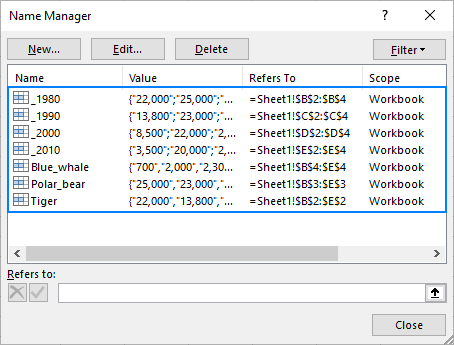
For our sample table, Excel automatically created only the row names. The column names have to be created manually because the column headers are numbers. To overcome this, you can simply preface the numbers with underscores, like _1990.
As the result, we have the following named ranges:
Part 2: Make a matrix lookup formula
To pull a value at the intersection of a given row and column, just type one of the following generic formulas in an empty cell:
Or vice versa:
For example, to get the population of blue whales in 1990, the formula is as simple as:
=Blue_whale _1990
If someone needs more detailed instructions, the following steps will walk you through the process:
- In a cell where you want the result to appear, type the equality sign (=).
- Start typing the name of the target row, say, Blue_whale. After you've typed a couple of characters, Excel will display all existing names that match your input. Double-click the desired name to enter it in your formula:

- After the row name, type a space, which works as the intersection operator in this case.
- Enter the target column name ( _1990 in our case).

- As soon as both the row and column names are entered, Excel will highlight the corresponding row and column in your table, and you press Enter to complete the formula:


Your matrix lookup is done, and the below screenshot shows the result:

That's how to look up in rows and columns in Excel. I thank you for reading and hope to see you on our blog next week!
Latest comments
I want to use the INDEX and VLOOKUP formula, but on a seperate sheet, instead of being in one.
There are pre-made stats on the 1st sheet, and stats I have to make in the 2nd sheet. The formulas must be in the 2nd sheet.
Hello Chris!
I recommend reading this guide: How to VLOOKUP across multiple sheets in Excel with examples.
For more info, please see also How to reference another sheet in Excel.
In your Table under INDEX MATCH MATCH, you have highlighted, for demonstration purposes, 22000, in pink ( the intersection of Polar Bear and the year 2000 ). My question is, IF I wanted to actually highlight the intersection value using CONDITIONAL FORMATTING, what would the formula be? Thank you.
Hello Michael!
You can use this conditional formatting formula for the cell range $B$2:$E$4:
=AND($A2=$H$1,B$1=$H$2)
The following tutorial should help: Relative and absolute cell references in Excel conditional formatting.
I have a table that looks very similar to this one used in the example. In my table, Column A is "Pipe Size" measured in inches (in your example, it's "Animal"), Row 1 is "Pipe Length" measured in feet (in your example, it's "Year"), and my table is populated with maximum gas loads that a pipe with the specific dimensions (size and length) can carry, measured in cubit feet per hour (CFH). In my situation, I know what the "Pipe Length" (ft) and the Load (cfh) is, and I'm wanting to match it to a specific size (inches) in Column A so that I can choose the correct pipe size. How would I be able to do that?
FOR EXAMPLE:
_________50_____100_____150___
__1____1,860___1,320___1,070__
__2____3,870___2,740___2,240__
__3____5,860___4,140___3,390__
Hello Jerad!
If I got you right, the formula below will help you with your task:
=INDEX(A2:A5,MATCH(G2,INDEX(B2:D5,,MATCH(G1,B1:D1,0)),0))
G1 = 100
G2 = 2740
The MATCH(G1,B1:D1,0) function determines the number of the required column. The INDEX(B2:D5,,MATCH(G1,B1:D1,0)) function returns all values from this column. Then the second MATCH function searches for the G2 value in this column and returns the corresponding value from column A using the INDEX function.
Hope this is what you need.
That was exactly what I was looking for, thank you!
Now, the next problem I'm running into is that the load isn't always going to be exactly the numbers found in the data range. The way we read the table is we determine the length of our pipe (B1:D1) and then look down the corresponding column to see where the load would fit. For example, I could have a 100 foot pipe length (C3) carrying a 2000 cfh load. I would choose to size the pipe at 2 inches (A4) because 2000 is too large for 1 inch (max of 1,320).
Can I modify the current formula to factor this in? Or is there another formula I can create in a helper table to help me assign the correct cfh (B2:D5) based on the correct column of pipe length (B2:B4 for 50 ft, C2:C5 for 100 ft, or D2:D5 for 150 ft)?
Hi Jerad!
When searching for the desired value in a column, you can use the XMATCH function instead of the MATCH function and the argument [match_mode]=1 - exact match or the next largest value. Try this formula:
=INDEX(A2:A5,XMATCH(G2,INDEX(B2:D5,,MATCH(G1,B1:D1,0)),1))
I hope my advice will help you solve your task.
I have a three column table (cells JA7 to JC10) which returns a value based on two criteria of Stage and colour (cells: JA3 to JC4), changing the stage or colour allows for comparisons and in the example below, the three colours are compared on the Stage 1 process.
IZ JA JB JC JE JF
3 Stage S1 S1 S1
4 Colour Yel Blu Grn Min Path
7 Brewery 8 5 4 4 {=INDEX($JA$4:$JC$4,MATCH(MIN(IF($JA7:$JC7>0,$JA7:$JC7)),$JA7:$JC7))}
8 Carpenter 4 4 4 4 {=INDEX($JA$4:$JC$4,MATCH(MIN(IF($JA8:$JC8>0,$JA8:$JC8)),$JA8:$JC8))}
9 Farmer 2 5 4 2
10 Blacksmith 3 14 8 3
And so on...
Column JE returns the minimum value for each item from row 7 onwards.
Column JF has an INDEX MATCH ARRAY formula to return the colour from row 5 based on the lowest value of the relevant line.
The formula is {=INDEX($JA$4:$JC$4,MATCH(MIN(IF($JA7:$JC7>0,$JA7:$JC7)),$JA7:$JC7))}
The problem I have and don't understand how to fix is why when the value in column JC is the lowest (as per line 7), the formula returns a value of #N/A instead of returning a colour from row 4. Whereas all the other results return the relevant "path colour" as the result.
Hi! Notice that you didn't use the Match_type argument in the MATCH function. Therefore, you are using an approximate match, in which the data must be sorted in ascending order. Use 0 for the Match_type argument. Read more in this guide: How to use MATCH function in Excel.
Hey,
You're an amazing help and make Excel super easy to understand so thank you!!
I just have one question...I work as an office manager for a bar and I'm trying to collect all my waiters/bartenders tips onto one page. Every night they write down on separate sheets (same workbook) how many tips they got and I want to be able to find them all in one easy table. How do I use IndexMatch across multiple sheets without having to rewrite the formula for each person and for each day?
The different sheets are labeled by the day of the month literally 1,2,3,4 etc through 31
Thank you so much!! You're so helpful!!
Alexa
Hello!
Here is the article that may be helpful to you: 3-D reference in Excel: reference the same cell or range in multiple worksheets.
I hope it’ll be helpful.
Hi, can you advise how to do a 2-way lookup in a table of numbers where the row and column headers are also numbers? So by inputting a number for the row header, and another number for the column headers, it would return a number from the table. Where the input row and column header numbers are not exactly matching the header number, it will look to the next higher header number and return the matrix number. Is that possible?
Hello!
If the number of row and column headings are in descending order, then you can use the formula:
=INDEX(B2:E4, MATCH(H1,A2:A4,-1), MATCH(H2,B1:E1,-1))
This is a great summary of all available methods for 2d lookups. Which method is the fastest for exact lookups?
Hello!
Here is the article that may be helpful to you: VLOOKUP in Excel - which formula is fastest?
Can you please advise how we can drag the results down to apply the formulae to multiple rows in a sheet.
I tried double clicking the square and also the copy pste special formulae in mass but does not seem to update the value until we double click in the formula itself.
Thank you,
Nikhil
Hello Nikhil!
I recommend instructions on how to copy a formula in Excel
Please also explain Xlookup and Xmatch which seem to replace not only vlookup/hlookup but also Index and Match
Hi Malcolm,
You are absolutely right. I've added the XLOOKUP formula to this tutorial. Also, we have a separate article that demonstrates all the abilities of this new function with formula examples: XLOOKUP function in Excel for vertical and horizontal lookup