The tutorial explains how to use COUNTIFS and COUNTIF formulas with multiple criteria in Excel based on AND as well as OR logic. You will find a number of examples for different data types - numbers, dates, text, wildcard characters, non-blank cells and more.
Of all Excel functions, COUNTIFS and COUNTIF are probably most often mixed up because they look very much alike and both are purposed for counting cells based on the specified criteria.
The difference is that COUNTIF is designed for counting cells with a single condition in one range, whereas COUNTIFS can evaluate different criteria in the same or in different ranges. The aim of this tutorial is to demonstrate different approaches and help you choose the most efficient formula for each particular task.
Excel COUNTIFS function - syntax and usage
The Excel COUNTIFS function counts cells across multiple ranges based on one or several conditions. The function is available in Excel 365, 2021, 2019, 2016, 2013, Excel 2010, and Excel 2007, so you can use the below examples in any Excel version.
COUNTIFS syntax
The syntax of the COUNTIFS function is as follows:
- criteria_range1 (required) - defines the first range to which the first condition (criteria1) shall be applied.
- criteria1 (required) - sets the condition in the form of a number, cell reference, text string, expression or another Excel function. The criteria defines which cells shall be counted and can be expressed as 10, "<=32", A6, "sweets".
- [criteria_range2, criteria2]… (optional) - these are additional ranges and their associated criteria. You can specify up to 127 range/criteria pairs in your formulas.
In fact, you don't have to remember the syntax of the COUNTIF function by heart. Microsoft Excel will display the function's arguments as soon as you start typing; the argument you are entering at the moment is highlighted in bold.

Excel COUNTIFS - things to remember!
- You can use the COUNTIFS function in Excel to count cells in a single range with a single condition as well as in multiple ranges with multiple conditions. If the latter, only those cells that meet all of the specified conditions are counted.
- Each additional range must have the same number of rows and columns as the first range (criteria_range1 argument).
- Both contiguous and non-contiguous ranges are allowed.
- If the criteria is a reference to an empty cell, the COUNTIFS function treats it as a zero value (0).
- You can use the wildcard characters in criteria - asterisk (*) and question mark (?). See this example for full details.
How to use COUNTIFS and COUNTIF with multiple criteria in Excel
Below you will find a number of formula examples that demonstrate how to use the COUNTIFS and COUNTIF functions in Excel to evaluate multiple conditions.
How to count cells with multiple criteria (AND logic)
This scenario is the easiest one, since the COUNTIFS function in Excel is designed to count only those cells for which all of the specified conditions are TRUE. We call it the AND logic, because Excel's AND function works this way.
Formula 1. COUNTIFS formula with multiple criteria
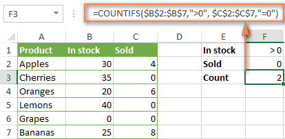
Suppose you have a product list like shown in the screenshot below. You want to get a count of items that are in stock (value in column B is greater than 0) but have not been sold yet (value is column C is equal to 0).
The task can be accomplished by using this formula:
=COUNTIFS(B2:B7,">0", C2:C7,"=0")
And the count is 2 ("Cherries" and "Lemons"):
Formula 2. COUNTIFS formula with two criteria
When you want to count items with identical criteria, you still need to supply each criteria_range / criteria pair individually.
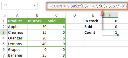
For example, here's the right formula to count items that have 0 both in column B and column C:
=COUNTIFS($B$2:$B$7,"=0", $C$2:$C$7,"=0")
This COUNTIFS formula returns 1 because only "Grapes" have "0" value in both columns.
Using a simpler formula with a single criteria_range like COUNTIFS(B2:C7,"=0") would yield a different result - the total count of cells in the range B2:C7 containing a zero (which is 4 in this example).
How to count cells with multiple criteria (OR logic)
As you have seen in the above examples, counting cells that meet all of the specified criteria is easy because the COUNTIFS function is designed to work this way.
But what if you want to count cells for which at least one of the specified conditions is TRUE, i.e. based on the OR logic? Overall, there are two ways to do this - by adding up several COUNTIF formulas or using a SUM COUNTIFS formula with an array constant.
Formula 1. Add up two or more COUNTIF or COUNITFS formulas
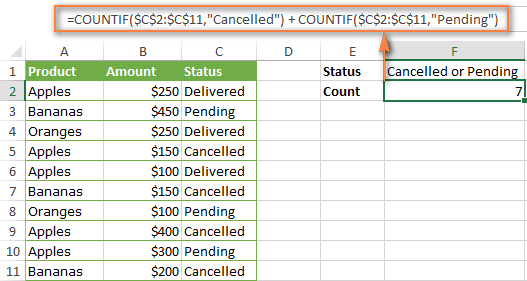
In the table below, supposing you want to count orders with the "Cancelled" and "Pending" status. To have it doen, you can simply write 2 regular Countif formulas and add up the results:
=COUNTIF($C$2:$C$11,"Cancelled") + COUNTIF($C$2:$C$11,"Pending")
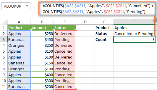
In case each of the functions is supposed to evaluate more than one condition, use COUNTIFS instead of COUNTIF. For example, to get the count of "Cancelled" and "Pending" orders for "Apples" use this formula:
=COUNTIFS($A$2:$A$11, "Apples", $C$2:$C$11,"Cancelled") + COUNTIFS($A$2:$A$11, "Apples", $C$2:$C$11,"Pending")
Formula 2. SUM COUNTIFS with an array constant
In situations when you have to evaluate a lot of criteria, the above approach is not the best way to go because your formula would grow too big in size. To perform the same calculations in a more compact formula, list all of your criteria in an array constant, and supply that array to the criteria argument of the COUNTIFS function. To get the total count, embed COUNTIFS inside the SUM function, like this:
In our sample table, to count orders with the status "Cancelled" or "Pending" or "In transit", the formula would go as follows:
=SUM(COUNTIFS($C$2:$C$11, {"cancelled", "pending", "in transit"}))
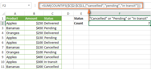
In a similar manner, you can count cells based on two or more criteria_range / criteria pairs. For instance, to get the number of "Apples" orders that are "Cancelled" or "Pending" or "In transit", use this formula:
=SUM(COUNTIFS($A$2:$A$11,"apples",$C$2:$C$11,{"cancelled","pending","in transit"}))

You can find a few more ways to count cells with OR logic in this tutorial: Excel COUNTIF and COUNTIFS with OR conditions.
How to count numbers between 2 specified numbers
By and large, COUNTIFS formulas for numbers fall into 2 categories - based on several conditions (explained in the above examples) and between the two values you specify. The latter can be accomplished in two ways - by using the COUNTIFS function or by subtracting one COUNTIF from another.
Formula 1. COUNTIFS to count cells between two numbers
To find out how many numbers between 5 and 10 (not including 5 and 10) are contained in cells C2 through C10, use this formula:
=COUNTIFS(C2:C10,">5", C2:C10,"<10")
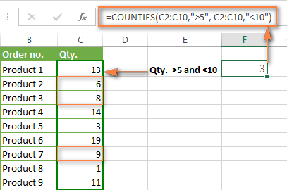
To include 5 and 10 in the count, use the "greater than or equal to" and "less than or equal to" operators:
=COUNTIFS(B2:B10,">=5", B2:B10,"<=10")
Formula 2. COUNTIF formulas to count numbers between X and Y
The same result can be achieved by subtracting one Countif formula from another. The first one counts how many numbers are greater than the lower bound value (5 in this example). The second formula returns the count of numbers that are greater than the upper bound value (10 in this case). The difference between the first and second number is the result you are looking for.
- =COUNTIF(C2:C10,">5")-COUNTIF(C2:C10,">=10") - counts how many numbers greater than 5 and less than 10 are in the range C2:C10. This formula will return the same count as shown in the screenshot above.
- =COUNTIF(C2:C10, ">=5")-COUNTIF(C2:C10, ">10") - the formula counts how many numbers between 5 and 10 are in the range C2:C10, including 5 and 10.
How to use cell references in COUNTIFS formulas
When using logical operators such as ">", "<", "<=" or ">=" together with cell references in your Excel COUNTIFS formulas, remember to enclose the operator in "double quotes" and
add an ampersand (&) before a cell reference to construct a text string.
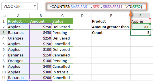
In a sample dataset below, let's count "Apples" orders with amount greater than $200. With criteria_range1 in cells A2:A11 and criteria_range2 in B2:B11, you can use this formula:
=COUNTIFS($A$2:$A$11, "Apples", $B$2:$B$11, ">200")
Or, you can input your criteria values in certain cells, say F1 and F2, and reference those cells in your formula:
=COUNTIFS($A$2:$A$11, $F$1, $B$2:$B$11, ">"&$F$2)
Please notice the use of absolute cell references both in the criteria and criteria_range arguments, which prevents the formula from being broken when copied to other cells.
For more information about the use of an ampersand in COUNTIF and COUNTIFS formulas, please see Excel COUNTIF - frequently asked questions.
How to use COUNTIFS with wildcard characters
In Excel COUNTIFS formulas, you can use the following wildcard characters:
- Question mark (?) - matches any single character, use it to count cells starting and/or ending with certain characters.
- Asterisk (*) - matches any sequence of characters, you use it to count cells containing a specified word or a character(s) as part of the cell's contents.
Tip. If you want to count cells with an actual question mark or asterisk, type a tilde (~) before an asterisk or question mark.
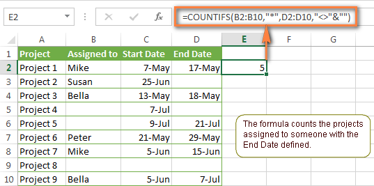
Now let's see how you can use a wildcard char in real-life COUNTIFS formulas in Excel. Suppose, you have a list of projects in column A. You wish to know how many projects are already assigned to someone, i.e. have any name in column B. And because we are learning how to use the COUNTIFS function with multiple criteria, let's add a second condition - the End Date in column D should also be set.
Here is the formula that works a treat:
=COUNTIFS(B2:B10,"*",D2:D10,"<>"&""))
Please note, you cannot use a wildcard character in the 2nd criteria because you have dates rather that text values in column D. That is why, you use the criteria that finds non-blank cells: "<>"&""
COUNTIFS and COUNTIF with multiple criteria for dates
The COUNTIFS and COUNTIF formulas you use for dates are very much similar to the above formulas for numbers.
Example 1. Count dates in a specific date range
To count the dates that fall in a certain date range, you can also use either a COUNTIFS formula with two criteria or a combination of two COUNTIF functions.
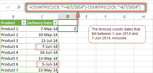
For example, the following formulas count the number of dates in cells C2 through C10 that fall between 1-Jun-2014 and 7-Jun-2014, inclusive:
=COUNTIFS(C2:C9, ">=6/1/2014", C2:C9, "<=6/7/2014")
=COUNTIF(C2:C9, ">=6/1/2014") - COUNTIF(C2:C9, ">6/7/2014")
Example 2. Count dates with multiple conditions
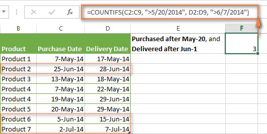
In the same manner, you can use a COUNTIFS formula to count the number of dates in different columns that meet 2 or more conditions. For instance, the below formula will find out how many products were purchased after the 20th of May and delivered after the 1st of June:
=COUNTIFS(C2:C9, ">5/1/2014", D2:D9, ">6/7/2014")
Example 3. Count dates with multiple conditions based on the current date
You can use Excel's TODAY() function in combination with COUNTIF to count dates based on the current date.
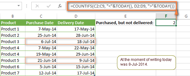
For example, the following COUNTIF formula with two ranges and two criteria will tell you how many products have already been purchased but not delivered yet.
=COUNTIFS(C2:C9, "<"&TODAY(), D2:D9, ">"&TODAY())
This formula allows for many possible variations. For instance, you can tweak it to count how many products were purchased more than a week ago and are not delivered yet:
=COUNTIFS(C2:C9, "<="&TODAY()-7, D2:D9, ">"&TODAY())
This is how you count cells with multiple criteria in Excel. I hope you will find these examples helpful. Anyway, I thank you for reading and hope to see you on our blog next week!
 by
by
1979 comments
In process of creating a 'master sheet' with sheet one including the formulas, and sheet 3 being the sheet where the data exported will be pasted into. Then sheet 1 will display the results as a summary so I'm pulling the data from sheet 3 onto sheet 1 based on certain criteria.
D Contains the location - hall, court, room, upper, lower etc..
E Contains the age - 6,7,8,9, etc...
I Contains a range of various activities in the one field - rugby club, football club, handball, tennis club, dance club..etc...
I want to pull one age group (6) from every location except two only (Hall and Court) only IF if I contains certain activities (Football, Tennis or Rugby) from sheet 3, into sheet 1. I enter the below formula in the cell I want the data in sheet one, and it returns zero. Zero is incorrect as when filtered there IS fields that are age 6, location other than Hall or Court that have done either football tennis or rugby.
=SUM(COUNTIFS(Sheet3!$E:$E,"6",Sheet3!D:D,"*Hall*",Sheet3!D:D,"*Court*",Sheet3!I:I,{"*football*","*tennis*","*rugby*"}))
Hello!
Without seeing your data it is difficult to give you any advice. Perhaps the age in column E is written as a number. Replace the text "6" with the number 6 (without quotes).
Hi. My data range (A1:B300) has reference numbers in A, and text lines in B. In C5, I type a word, and I want to see in D5 the row(s) from the range having the word. COUNTIF tells me the number of times the word occurs in the range. Is there a formula I can use in D5, so that I can avoid having to use data filter on the range. Thanks.
Hello!
To get conditionally from a range of rows, you can use the FILTER function. You can find instructions and examples in this article.
I hope it’ll be helpful. If something is still unclear, please feel free to ask.
Hi - I need help with creating a tally based on date and time frames. I am trying to calculate how many flights are within a specific day in a column, but within each day, I need it broken up in intervals of time. For instance, I need every hour of each day. Let's say I am looking at 300 flight itineraries (all arriving within a 3 day period 4/2/2022, 4/3/2022, and 4/4/2022). I need to look at each day specifically and be able to break down how many people arrive at for example, 1 - 1:59 pm, 2 - 2:59 pm, 3 - 3:59 pm and so forth. I understand how to do the count ifs for a time frame, but how is there a way to include the conditional for the date.
Hello!
If the cell contains the date and time in the mm-dd-yyyy hh:mm:ss format, then you can write the condition something like this:
">="&(DATE(2022,4,2)+TIME(13,0,0))"
Please check out this article to learn how to insert time using the Excel TIME function.
Hello, I'm trying to figure out how to find matches between a cell containing multiple comma separated numbers and another cell containing multiple comma separated numbers.
Here is my example, cell 1 contains 12345, 12346, 12347, 12348,
cell 2 contains 54321, 12345, 65432, 23456, 12347
I want to do two things -
1. provide a true/false 1/0 answer in the cell if any number in cell 1 shows up in cell 2
2. in another cell count the number of matches between cell 1 and cell 2
I have had to break out the imported data and separate it out by commas manually, and it is time consuming. I figured I would reach out to people who are much smarter than me to get some insights.
Thanks for your time,
Jeremy
Hello!
You can split text by rows using the Split Text tool. Then compare 2 columns and determine the number of duplicates as described in this tutorial.
Unfortunately, this problem cannot be solved by ordinary Excel formulas. It is possible to write a custom VBA macro
Hi,
I'm trying to count data in an entire table based on a date, then return the total of this. This table has multiple rows for data from 01/2/3/4 of January and will continue.
The formula works whenever I change the date however, I want to count of data from another column, based on each [date].
Note these are all in the same table with rows appended each day.
For clarification I want to return the total of [Date] + return me total of [Status] on [Date]
Hello!
As I understand the problem, then you should use the SUMIFS function. You can learn how the SUMIFS function works with dates in Excel in this article on our blog.
Hi,
I was working on some calculations but unable to find the solution.
I want to count the number of days on which the minimum balance is maintained
For Example
On 1.12.21 on 2.12.21 on 3.12.21 Minimum Balance Remarks - Formula required
75 70 50 60 (Min balance maintained - 2 days)
50 60 45 70 (Min balance maintained - 0 days)
45 20 35 10 (Min balance maintained - 3 days)
Hello!
Based on your description, it is hard to completely understand your task. However, I’ll try to guess and offer you the following formula:
=COUNTIF(A1:C1,">"&D1)
If this is not what you wanted, please describe the problem in more detail.
Greeting,
I have datasheet i want to count the Age categories, related local and female.
Mean how many local female we have above 19 years to 48 years. below formula can't working.
=COUNTIFS('Datasheet'!E36:E139,"female",'Datasheet'!G36:G139,"19-48",'Datasheet'!H36:H139,"local")
Hi!
Instead of G36:G139,"19-48", use two conditions: G36:G139,">19", G36:G139,"<48"
I'm not seeing your data, but I think that will be helpful.
Hi
I am creating a spreadsheet for a sales tracker. I have a weekly tab (x13) and I have multiple drop down options (Current account, saver, mortgage etc) in one column and the next over the date the account was opened. I am trying to total up in another tab the total number of say current accounts keyed but only once the week number has been added else it doesnt count. So the other tab has a list of all the product options with number opened for a total of 13 weeks (quarterly total). Help please! So stuck!
Hello!
Unfortunately, without seeing your data it is difficult to give you any advice. You need to use COUNTIFS as recommended in this article. The criteria are the invoice date in the date range (there is an example above) and the product code.
I have a CSV file downloaded with info about orders. I want Excel to somehow count the number of orders of each type per person.
i.e. Sherry ordered 3 Chicken pies, and 2 Butter Tarts,
Joanne ordered 2 Butter Tarts,
Marie ordered 2 Beef pies and 2 Butter tarts
and Bill ordered 3 Beef Pies, 3 Chicken etc.
Currently it looks like this: (I didn't know how to attach a screen shot so I just separated the column info by /
Order number 1/Sherry/chicken/address/phone #
Order number 2/Sherry/chicken/address/phone #
Order number 3/Sherry/chicken/address/phone #
Order number 4/Sherry/butter tart/address/phone #
Order number 5/Sherry/butter tart/address/phone #
Order number 6/Joanne/butter tart/address/phone #
Order number 7/Joanne/butter tart/address/phone #
Order number 8/Marie/beef/address/phone #
Order number 9/Marie/beef/address/phone #
Order number 10/Marie/butter tart/address/phone #
Order number 11/Marie/butter tart/address/phone #
Order number 12/Bill/beef/address/phone #
Order number 13/Bill/beef/address/phone #
Order number 14/Bill/beef/address/phone #
Order number 15/Bill/chicken/address/phone #
Order number 16/Bill/chicken/address/phone #
Order number 13/Bill/chicken/address/phone #
The way that the Excel sheet works now, I have to count the number of items of each kind per person... Too much work when there are many items (sometimes we have up to 50) and too big a margin for error (If we miscount or count someone else's order by accident.)
Any ideas how I can make this work? (I'd be ok if each item that they ordered had it's own line beside the name.
Hello!
You can get a list of orders for an individual person using the FILTER function.
To count orders of each type per person, I recommend using a pivot table.
I hope this will help, otherwise please do not hesitate to contact me anytime.
Alexander,
Sorry for the additional email. My formula below worked, but when I applied to all months in the year, it wasn’t counting correctly for each month. When I applied the correction below (and adjusted the date range for each month), it counted correctly.
=SUM(COUNTIFS(daterange,">=02/01/2021",daterange,"<03/01/2021",schoolrange,{"school 1","school 1","school 2", "school 2","school 3","school 3"},subjectrange,"Art",projectstatusrange,{"finished","nearly finished","finished","nearly finished","finished","nearly finished"}))
Alexander
Thank you for your help. Prior to requesting, I did look through the prior chats before requesting advice. Thank you for the formula provided. Initially the formula was not picking up any values, but was returning a 0. I tried substituting named ranges for the cell ranges in the provided formula and that did the trick.
=SUM(COUNTIFS(daterange, ">=01/01/2021",daterange, "<02/01/2021",schoolrange,{"school 1","school 2"},subjectrange,"art",projectstatusrange,{"finished","nearly finished"}))
Where daterange is the specified cell range for the dates, schoolrange is the specified cell range for school numbers, subjectrange is the cell range for the various subjects, and projectstatusrange is the cell range for the various project status’.
I appreciate your expertise and help. I use and reference your blog and find it to be one of the better and more responsive blogs.
Best regards-
Good day,
I’m struggling with a Countifs formula and could use your help.
I have two tabs-formula is in tab/sheet 1, data table is in tab/sheet 2.
I’m trying to determine the number of times one of two project status appear based on certain conditions:
On tab/sheet 2, the data is set up as follows:
Column 1 is School 1, School 2, School 3
Column 2 are the subjects: Art, math, science, language, etc…
Column 3 is the project status: not started, started, in process, nearly finished, finished
Column 4 is the date of the entry/status update
I am trying to write the a formula that accomplishes the following:
The number of projects between date range >=01/01/2021 to <02/01/2021 for just the the art classes from either school 1 or school 2 that are in either a “nearly finished” or “finished” status
I’ve tried using if(and combined with a count if, but I continue to get #value errors.
Any help is greatly appreciated.
Hi!
Have you tried the ways described in this blog post? I hope you have studied the recommendations in the tutorial above. It contains answers to your question.
Something like this formula:
=SUM(COUNTIFS(D2:D9, ">=01/01/2021", D2:D9, "<02/01/2021",A2:A9,{"school 1","school 2"},B2:B9,"art",C2:C9,{"finished","nearly finished"}))
I have to calculate child spaces for a month. I used S as sick. We allow 5 sick days per child per month to be counted towards compensation, anything over 5 days is not counted. The formula I used to count days for present was =COUNTIF($B11:$AF12,"P"). But I cant figure out the S days to minus the 5 allowable days. Any help would be greatly apprecied
Hi!
I’m not sure I got you right since the description you provided is not entirely clear. However, it seems to me that the formula below will work for you:
IF(COUNTIF($B11:$AF12,”S”)>5,5,COUNTIF($B11:$AF12,”S”))
If this is not what you wanted, please describe the problem in more detail.
Hey there,
I have a data sheet with columns indicating characteristics that are labelled with numbers to indicate which characteristic. 1: Black 2: Yellow 3: Brown 4: White 1: Cat 2: Dog
I would like to find out which cells in the spreadsheet have the two matching characteristics.
eg. "black" "dog" So, the end goal is to have 1 number added to the answer box for each person in the survey who owns a dog that is black.
=countif(Data!R1:R99, "2", Data!Q1:Q99, "1")
Would you care to tell me what is wrong about my formula?
Hello!
To count on multiple conditions, use the COUNTIFS function. Please read the above article carefully.
Thank you so much!
The different between plural and non plural is what was holding me back.
This has helped me immensely and I am happy that you responded promptly.
Hello There,
I have multiple columns, example:
Code ; Environment; value
xyz; Dev;1
xyz; SIT;1
xyz; PAT;1
ABC;DEV;1
PQR;PROD;1
Now, i need to take only values which has Dev and either SIT or PROD or PAT, flag them True. if it is just Dev only they flag them False.
Need your guidance. thank you
Hello!
You can use the IF function with multiple conditions. I cannot offer you a formula, since your conditions are incomprehensible to me. On the first line, both TRUE and FALSE are true. If not, give an example of the result you want.
Hi,
When using dates as the criteria arguments, do you have always specify in US date numerical format rather than UK equivalent?
I live in the UK and so the convention we use to convert 1st June 2015 to numerical format is "01/06/2015". In the USA this would be 06/01/2015.
Does excel functions only work with the later?
Thank you so much for this!
Hi, please help! I have 2 columns, Column A "Date" and B is status if "Passed/In Progress".
I need to count the number of "Passed" using a date range provided in a cell. Here's a sample:
COLUMN A. Column B. Column C. Column D Column E
10/1/2021 Passed 10/1/2021 10/30/2021 2
10/5/2021 In-Progress
10/10/2021. Passed
11/01/2021 Passed
My sample seems wrong didn't know spaces will be deleted after posting.
Column A "Date", Column B "Passed/InProgress", Column C and D "Date Range", Column E "Count Passed"
I need to know what formula am I going to use on Column E. Thank you so much!
I just found out the answer it's:
=COUNTIFS($B$2:$B$6,">="&$C$2,$B$2:$B$6,"<="&$D$2,$A$2:$A$6,"Passed")
Thanks!
Hello!
Please re-check the article above since it covers your task.
Here is one more article that may be helpful to you: COUNTIF formulas for dates.
I hope I answered your question. If something is still unclear, please feel free to ask.
Hi, I'm not sure how to put this in the formula and not even sure what function I need to use, can someone help me, please?
I have 2 sheets named and with column names below
Sheet 1 Name: Est Sheet (with data)
Column A: Facility Name (with data)
Column B: Department (with data)
Column C: Est Asset (with data)
Column D: Actual Asset (data needs to come from Sheet 2)
Sheet 2 Name: Asset Located
Column A: Asset Name
Column B: Facility Name
Column C: Department
I would like to pull out the total numbers of asset per facility and department from Sheet 2 and show it on Column D of Sheet 1.
How do I count the number of assets on each facility and department and pull out the sum to Column D of Sheet 1?
Help, please. Thank you!
Hello!
I kindly ask you to have a closer look at the article above.
Counting values according to two conditions:
=COUNTIFS(Sheet2!B2:B100,Sheet1!A2,Sheet2!C2:C100,Sheet1!B2)
can someone help me to get below result, count # of material based on two conditions.
detail
work order Date material
100 12-Oct ab
200 13-Oct cd
100 12-Oct ef
result
work order Date material
100 12-Oct 2
Hi!
You can use the formula
=COUNTIFS(A2:A100,100,B2:B100,DATE(2021,10,12))
If you need to calculate the unique values of materials, then I recommend the article: How to count unique values in Excel with criteria.
I hope my advice will help you solve your task.
I imported two separate reports into either same sheet or different sheets. Each report have in separate columns, b and ac, matching and unmatching number values. I need to identify a formula to return matching value from Report 1 (column b) Report 2(Column ac) to calculate total amount from Report 2 (Column ad if column b and column ac then match column e to column v and place total amount in column w) that matches the value from table array (column v match column e). As you can see below, in the table array (column v, data 3) matches from Report 1(column b, rev 3 and rev 7) with Report 2(Column ac, rev3) where the table array (data 3) calculates the total value to match all the criteria's of table 1 and table 2 and places the total amount from Report 2 (Column ad, $1.00 and $4.00). I hope this makes sense as this is difficult to explain.
Report 1 Table Array Return Value Report 2
Column b Column e Column v Column w Column ac Colum ad
rev1 Data1 data1 ($0.00) Rev3 $1.00
Rev2 Data6 data2 ($0.00) Rev4 $3.00
Rev3 Data3 data3 ($5.00) Rev5 $10.00
Rev4 Data4 data4 ($3.00) Rev7 $4.00
Rev5 Data2 data5 ($0.00) Rev10 $1.00
Rev6 Data1 data6 Rev12 $2.00
Rev7 Data3 data7 Rev15 $3.00
Hello!
Your request goes beyond the advice we provide on this blog. This is a complex solution that cannot be found with a single formula. If you have a specific question about the operation of a function or formula, I will try to answer it.
Hey,
I'm trying to use COUNTIF to look at 2 different collums and if both of the values are true to count, this is my formula but it is not working;
=COUNTIF('2021 Requests'!C6:C440, "Granted",'2021 Requests'!D4:D440,"07/01/2022")
Any help would be appreciated.
Needs to be COUNTFS not COUNTIF
also the range of C should be the same size as the range of D
so EX.
=COUNTIFS('2021 Requests'!C4:C440, "Granted",'2021 Requests'!D4:D440,"07/01/2022")
I have three colms
A B C
Loss amnt reason
Yes 100 Retrun
i have tried countifs( B1:B10,"<100",C1:C10,"return") but actual picture will be on the basis of Loss ( Yes or No). what is the formula for that.
Hi!
If you want to calculate the amount of losses, then use the SUMIFS function.
=SUM(COUNTIFS(D24,"*P*"),(COUNTIFS(D55,"*P*")),(COUNTIFS(D104,"*P*")))
I'M TRYING TO GET THE SUM OF DIFFERENT CELLS IN SAME COLUMN THAT IS MY SAMPLE FORMULA HOW CAN I SHORTEN IT IF I HAVE MORE THAN 20 LIST.. FOR THE FORMULA ABOVE THAT IS FOR MY FOREMAN THEY ARE "P" BECAUSE THEY ARE PRESENT I WANT TO COUNT THE PRESENT NO NEED FOR THE ABSENTS BUT MY HELPER IS 20 AND MORE I WANT TO TRY AND SHORTEN IT . I ALSO HAVE A FORMULA FOR MY 11 CARPENTERS
=SUM(COUNTIFS(D30,"*P*"),(COUNTIFS(D35,"*P*")),(COUNTIFS(D39,"*P*")),(COUNTIFS(D40,"*P*")),(COUNTIFS(D67,"*P*")),(COUNTIFS(D68,"*P*")),(COUNTIFS(D70,"*P*")),(COUNTIFS(D75,"*P*")),(COUNTIFS(D76,"*P*")),(COUNTIFS(D85,"*P*")),(COUNTIFS(D106,"*P*")))
IF YOU CAN HELP ME THAT WOULD BE A BIG HELP
TIA
ANW I ALREADY GOT THE ANSWER TYVM <3
=COUNTIFS(D21:D118,"P",C21:C118,"CARPENTER")
Hello!
If your data is written in separate cells, you need to specify each cell separately. To reduce the formulas, you need to change the data table.
Thank you ! I did it by using countifs with multiple criteria
I did it by reading your article word by word haha thank you !
Hello there! First I'm working on a spreadsheet where there are sometimes multiple rows for a single machine, and sometimes there is only one, I'm trying to get a function that works in a similar way to the countifs, but instead of resulting the number of cells it gives me the "name" or "address" of the cell, Example: =countifs(J61423:J61463;J61460; K61423:K61463;K61460) -> It results "2" but what I want is "(J61459; J61460)" which are the cells that I need.
For extra clarity: I'm asking if it is possible to do this by any function or mean, not necessarily using countifs, this function would simply work in a similar way to it. Is there something like that that I can use?
Hello!
You can get the cell address using the ADDRESS function. You can find the examples and detailed instructions here.
Can you please help? I am working from two tables. First table has a list of student group codes and the course department codes. The second table has a list of all the student names/their student group codes/course/department/course department codes, all in different columns. From table 2, I'm trying to do a count of total students in each student group codes in table 1 that shows up in each course department codes. Same student group code can belong to different dept codes.
Raw data is in Table 2 in different columns. Example of columns header below
Table 1
Stu_Grp Dept Dept Codes Dept
106100 2 Org_2200 Business
107100 2 Org_2201 Management
105100 4 Org_2400 Law
102100 6 Org_2600 Marketing
102200 8 Org_2800 Finance
104200 4 Org_2400 Law
104300 2 Org_2200 Business
104400 2 Org_2201 Management
105100 7 Org_2700 Accounting
Table 2
Student NameStud_Grp Dept 2 Codes Dept Description Dept 4 Codes Description Dept 6 Codes Descript
Hello!
Unfortunately, without seeing your data in Table 2, it is difficult to give you any advice. I think you need to use the COUNTIFS function. If you have specific questions about the formula, I will try to answer them.
Hello! I'm in need of a bit of help please :)
In my worksheet, I have a drop down list in row G10:CK10 for "Completed", "Ongoing", "Cancelled".
In the column G17:Y50, I have names of speakers, some of which are repeating names.
I would like to count the number of "Completed" events for each speaker. I have tried the COUNTIFS function, but unfortunately using the formula below it keeps returning as a VALUE error:
=COUNTIFs(G10:CK10, "Complete", G17:Y50, "Linda").
I would if you would be able to help?
Many thanks!
Hello!
You have different range sizes for the criterion and for the count, so the COUNTIFS function cannot be used.
If I got you right, the formula below will help you with your task:
=SUM(($B$10:$J$10="Complete")*($B17:$J50="Linda"))
I hope it’ll be helpful.
This is absolutely perfect! Thank you very much for your help!!
hello,
I need a little help :)
I have a excel file with some documents with bill ID and Dealer ID. I want to count number of dealer who has sold each product. Can you help me find a formula as detail below:
Date dealerID Bill Number Product ID Amount
23-03-21 68345307 21016501146004 5 1500
23-03-21 68345307 21016501146004 6 500
23-03-21 68345307 21016501146004 7 1000
23-03-21 68345307 21016501146004 8 1000
23-03-21 68345307 21016501146004 9 1000
24-03-21 963949731 21016601151003 0 100
24-03-21 963949731 21016601151003 2 100
24-03-21 963949731 21016601151003 5 100
24-03-21 963949731 21016601151003 7 100
24-03-21 963949731 21016601151003 9 100
25-03-21 99336636 21016701145002 0 2000
Product ID Total Amount No. Bill No. Dealer
0 2100 2 ?
1 0 0 ?
2 100 1 ?
3 0 0 ?
4 0 0 ?
5 1600 2 ?
6 500 1 ?
7 1100 2 ?
8 1000 1 ?
9 1100 2 ?
Hello!
I recommend using the information in this article: Count unique values with criteria.
The formula is something like this:
=IFERROR(ROWS(UNIQUE(FILTER(B2:B12,D2:D12=H2))), 0)
H2 -- Product ID
B2:B12 -- Dealer ID
Hi,
please see below, i have 2 columns, first one are the jobs working on, second column is phases in the job, how i can sum, count each phase for this job repeating in the column? different jobs may have same phases, so need phase column be dependant on job column... please help
job phase
3156 112
3156 541
3137 541
3156 99020
3156 99020
3137 541
3137 541
3156 99020
wip wip
Hi!
I do not quite understand what you want to calculate. How to calculate the number of phases for each job is described in this article above. If you need to calculate an amount with multiple conditions, use the SUMIFS function.
Hello, I've searched multiple threads and cannot find a combination that might help my scenario. I'm using COUNTIFS successfully. Ex. =COUNTIFS(A:A,"employee",C:C,"product") But how can I add a third criteria that counts ''repair order" only once if it is replicated? I think the correct term is 'Distinct'.
Here is a small sample where the result = 6
However Repair Order 206189150 is duplicated so the desired result is = 5
employee repair order product
318 206188973 ABLAST
318 206189055 ABLAST
318 206189150 ABLAST
318 206189150 ABLAST
318 206189160 ABLAST
318 206189188 ABLAST
I hope this is clear and I'm sorry about formatting.
Thanks in advance! - Craig
Hello!
I recommend reading this guides: Count unique rows in Excel and How to count unique values in Excel with criteria. Use a formula like this:
=ROWS(UNIQUE(FILTER(A1:C6,A1:A6=318)))
I hope it’ll be helpful.
Hi there,
second day in a row, sorry about that.
Is there a way to search across multiple sheets (i know that is a VLOOKUP) but to return values from the search?
In this case I have data from various cities, (all sheets are the same layout) and i want to look up the Sector (coloum D) for say "Construction" and return the total cost across all sheets (column F)
Hello!
If the “Construction” value is written in different positions on each sheet, then I recommend using the Consolidate Sheets tool.
You can use the SUMIF function for each sheet and then summarize the results.
Hi there, Im trying to return a result if one 'phrase' is met, and then one do have a difference result if one of 5 others.
I had a try but seem to have failed miserably with the second criteria/calculation
please help
IF(SUM(COUNTIF(E3,{"*In work as a result of LVP*"})),B3,""),(SUM(COUNTIF(E3,{"*In work through other means*","*Awaiting a start date*", "*Out of work*", "*Health Condition*", "*Other*"})),(B3-(B3*2)),"")
Hi,
if I understood the problem correctly, try this formula:
=IF(SUM(--ISNUMBER(SEARCH("In work as a result of LVP",E3))),B3, IF(SUM(--ISNUMBER(SEARCH({"In work through other means","Awaiting a start date", "Out of work","Health Condition","Other"},E3))), (B3-(B3*2)),""))
Hi there,, Thankyou SSOOO much, thats amazing
I am trying to use the Countifs to count the number of cells that fall within a specific date range and are between two values.
Example: If I want to know how many cells are between 40 and 60 (Cell E) and between the dates of 3/1/21 and 3/31/21 (Column A)
Formula I have been trying to get to work is
=COUNTIFS($A$4:$A$1000000, ">="&G5, $A$4:$A$1000000, "<="&H5,$E$4:$E$1000000, "&=40")
however, its returning over 27K as the count. I know I only have 1365 cells in this date range.
Any help would be appreciate.
Thanks
Hi!
Please use the following formula:
=COUNTIFS($A$4:$A$1000000, “>=”&G5, $A$4:$A$1000000, "<="&H5,$E$4:$E$1000000, ">="&40,$E$4:$E$1000000, "<="&60)
I have a need for a 3rd criteria. Using your example I would want it to countif Susan has a project, with a start date, but no end date. The example I am looking at is under "How to use COUNTIFS with wildcard characters".
Hi Bryan,
Simply, use 3 range/criteria pairs:
=COUNTIFS(B2:B10, "susan", C2:C10, "<>"&"", D2:D10,"")
if having a range of cells (D3:M37) where certain cells contain text: Yes, No, Maybe, how to return a result in another cell as the Yes or No or maybe correspond to a name in column B, for example, cell F3 has a NO the result (wanted to appear in P4) should be B3 name.
Hope this make sense
Thank you.
Hi, I've been stuck at this for hours.
I'm supposed to Input either a "Yes" or "No" or blank for 12 columns in a single row.
However I need a formula to Prioritize "NO" over the other answers.
But:
1. if there isn't "NO", but there's "YES" and blanks, then the cell should reflect "YES"
2. If there isn't "NO" or "YES", the cell should be blank
I tried Match and CountIF formula but i can't get the result i need.
Any help would be greatly appreciated!
Could you please help me
If in One Column I have Y 2,Y 1,Y 6, N3 is there a way that i can sum the Numbers only
Hello!
If I understand your task correctly, the following formula should work for you:
=SUM((IF(ISNUMBER(--MID(CONCATENATE(A1,A2,A3,A4),ROW($1:$100),1)),--MID(CONCATENATE(A1,A2,A3,A4),ROW($1:$100),1),"")))
or
=SUM((IF(ISNUMBER(--MID(CONCAT(A1:A4),ROW($1:$100),1)),--MID(CONCAT(A1:A4),ROW($1:$100),1),"")))
I hope it’ll be helpful.
Hi,
I've been spending days on getting the formula right, but still uncertain how to get the right info.
I've got two columns with different dates: Start Date (A) & Resignation Date (B).
Currently using =COUNTIFS(A3:A143, "=",B3:B143,"=>1-90" but doesn't seem to give the right answer.
I would like to calculate how many people are resigning within 3 months, between 3-6 months, between 6-12 months. Any idea how the formula will look like?
Thanks.
Hello!
To calculate how many people are resigning within 90 days, use the formula
=SUMPRODUCT(((B1:B15-A1:A15)<90)*((B1:B15-A1:A15)>0))
I hope it’ll be helpful.
Hi Alexander,
Thank you so much, this is definitely working!! :)
Regards,
Cindy
=SUM(COUNTIFS('SACE stg 2 2017'!F:F,OR('SACE stg 2 2017'!$F$1253,'SACE stg 2 2017'!$F$1256,'SACE stg 2 2017'!$F$1478,'SACE stg 2 2017'!$F$1484,'SACE stg 2 2017'!$F$1490,'SACE stg 2 2017'!$F$1495,'SACE stg 2 2017'!$F$1502),'SACE stg 2 2017'!G:G,'Lingustics subject'!A3), COUNTIFS('SACE stg 2 2017'!F:F,OR('SACE stg 2 2017'!$F$1253,'SACE stg 2 2017'!$F$1256,'SACE stg 2 2017'!$F$1478,'SACE stg 2 2017'!$F$1484,'SACE stg 2 2017'!$F$1490,'SACE stg 2 2017'!$F$1495,'SACE stg 2 2017'!$F$1502),'SACE stg 2 2017'!G:G,'SACE stg 2 2017'!$G$55))
This is my formula, I used the or statement to select a wide range of data that could include in a range, but it seems to didn't work. How can I fix this?
Hi!
It is very difficult to understand a formula that contains unique references to your workbook worksheets. Hence, I cannot check its work, sorry.
Hi,
I have following large set of data.
Catalogue Lot Count
HBI66545 1320000531 2
HBI66545 1320000531 2
HBI66545 1320000531 2
HBI66545 1319000101 2
HBI66545 1320000531 2
HBI66545 1320000531 2
HBI66545 1319000101 2
I have used this formula to count.
=SUM(B2=$B$2:$B$18,(1/COUNTIFS($A$2:$A$18,$A$2:$A$18,$B$2:$B$18,$B$2:$B$18,$C$2:$C$18,$C$2:$C$18)),0)
But my problem is I would need sum of Catalogue and Lot which should be 5 for 1320000531 and 2 for 1319000101. Could you help me solving this?
Thanks heaps
Hi!
Your explanations are not very clear. I am assuming that you want to count the number of occurrences of a value. For example 1320000531.
A simple COUNTIF formula is suitable for this, as described in this article.
If this is not what you wanted, please describe the problem in more detail.
How can I use CountIFs function while counting the data of specific individual for a specific range of dates. Example, I have list of names in column A (from A2 to A20), their daily working hours is between column C2 to AF20 (31 days). Now I want to calculate number of days each individual did less than 5 hours shift, number of days an individual was not present in that month, total working days etc. I know I can do all these calculations for each individual at the end of the last column but I am pulling this data at another sheet and the names may not be in same order.
Is there any other way other than CountIFs? Any help would be appreciated.
Hello!
To calculate the number of days with more than 5 working hours, you can use the formula
=SUMPRODUCT((Sheet1!$A$2:$A$20=$A$2)*(Sheet1!$C$2:$AF$20>5))
where cell A2 -- Name.
Please have a look at this article - Excel SUMPRODUCT function with formula examples
I have a spreadsheet that i want to return a count across a row if two conditions are met.
please whats the best way to write this code =if(AC3="Reject", AF3="vendor", Count(f3:Y3))
when i wrote this code, i noticed the ones that met the condition only returned "True" instead of counting across the row, see below.
Number of Rejects Due Supplier
1
TRUE
5
TRUE
TRUE
Hi!
If I understand your task correctly, the following formula should work for you:
=IF(AND(AC3="Reject", AF3="vendor"), COUNT(F3:Y3))
I hope it’ll be helpful.
Hello Alexander,
Yes this was helpful, but i like to have 0 for the once that didnt meet the condition instead of "false"
Actual expected
false 0
3 3
False 0
4 4
1 1
Hi!
I recommend reading how the IF function works and correcting the formula. It’s very simple.
Hi - i am trying to count the number of dates in a date range and using a countifs formula. Such as:
COUNTIFS(N:N,">="&B2,N:N,"<="&B3)
Where B2 refers to Start Date & B3 refers to end date (e.g. B2 = 01/04/2021 and B3= 30/04/2021)
It is calculating the dates but is not including the start(B2) and end date(B3) rather just the data greater to or less than the start(B2) and end dates(B3)
Do you know how to include the data for the dates noted in B2 and B3?
Thanks
Hello!
I used your formula and got no errors. Perhaps your dates in column N are written as date and time.
Hi , i am looking formula to rid of all the duplicates & the originals in comparision data . some duplicates starts with "."
Just example
Existing:
a123.com
.a123.com
Comparing with
a123.com
I need to remove all "a123.com" . i have sheet of of 10000+ in existing & comparing have "2000+" .
how to remove the duplicates even it have "." in starting .
i am using the formula of -=IF(COUNTIF(A:A,A2)=1,0,1). it detecting the exact duplicates but not catching any thing with "." in starting.
Hello!
If you need a partial text match, I recommend using this instruction: How to count cells with certain text (partial match).
I hope I answered your question. If you have any other questions, please don’t hesitate to ask.
Hi Alexander,
I'm trying to create a formula for this scenario. I have two columns, in each column there are only two texts that can be selected from a drop down (I'll call them "Text123" and TextABC"). I would like to create a formula that counts the total results for each for both columns, however, if "TEXT123" was selected in row 1 for both columns 1 & 2, I would only need to count it as one, not 2. How do I create a formula telling excel to count it only once per row, but for two columns total.
Thanks so much in advance.
Hello!
If I got you right, the formula below will help you with your task:
=SUM(--(A1:B10="TextABC"))+SUM(--(A1:B10="Text123"))-SUM(--(A1:A10&B1:B10="Text123Text123"))
Hi Alexander,
My spreadsheet is quite simple, it has 3 columns.
Column one has type of activity. (for ease of use, we can say Walk, Run & Swim)
Column 2 has only 2 options "1st Pass" or "Not 1st Pass".
Column 3 has a date.
I need to have a count depending on the month & year.
I can get each activity & whether its 1st pass or not 1st pass. Input is from Row 3 downwards.
My problem is when I am trying to choose month = 8 & year = 2021.
Formula just on basic Walk * 1st pass is =COUNTIFS(Applications!$A$3:$A$974,"Walk",Applications!$B$3:$B$974,"1st pass")
I have a table which splits each activity (rows) and months (columns). I would like to return the count of 1st pass walks in each month & year? I have used Month & Year function with SUMPRODUCT, but they seem to cause issues with COUNTIFS.
I was trying (year I am wanting to use is in C1 so I can change review previous years- in below formula looking for August in the year provided in cell C3):
=COUNTIFS(Applications!$A$3:$A$974,"Walk",Applications!$B$3:$B$974,"1st pass",Applications!$C$3:$C$974,MONTH(Applications!$C3:$C974)=8,Applications!$C$3:$C$974,YEAR(Applications!$C3:$C974)=$C$1)
Messed up down the bottom:
I was trying (year I am wanting to use is in C1 so I can change review previous years- in below formula looking for August in the year provided in cell C1):
Hello!
If I understand your task correctly, the following formula should work for you:
=SUMPRODUCT(--(A1:A10="Walk"),--(B1:B10="1st Pass"),--( YEAR(C1:C10)=2021),--( MONTH(C1:C10)=8))
If this is not what you wanted, please describe the problem in more detail.
Thanks Alexander,
I am looking to be able to return a result through countifs while searching for specific month & date within the range.
Just say date values fill up cells A1:A10.
How would I write a countifs formula searching for the month 8 (Aug) and year 2021?
Thank you for your review.
Hi!
The COUNTIFS function compares each value in a range against a criterion. You are comparing a date with a month number. Therefore, your COUNTIFS formula will not work.
Hello ,
Can u help me to set the below formula
=IF(B4:B30,"Purchase Invoice",COUNTIFS(K3:K30,"1-20"))
Thanks in advance
Hello!
The IF function does not work with ranges. Please describe your problem in more detail. It’ll help me understand it better and find a solution for you.
- C1 C2 C3 C4
R1 Apr-21 Apple 10 Delivered
R2 Apr-21 Bannana 15 Pending
R3 Apr-21 Oranges 23 Delivered
R4 May-21 Apple 12 Pending
R5 May-21 Apple 45 Delivered
R6 May-21 Bannana 27 Cancelled
R7 May-21 Oranges 24 Pending
R8 Jun-21 Apple 11 Cancelled
R9 Jun-21 Apple 10 in Transit
R10 Jun-21 Bannana 26 Cancelled
need to filter in c1 ( apr, june), then c2 (oranges, apple), then c4 (delivered, pending); the answer should be 2
I need countifs in single formula for above; please advise
Hello!
I believe the following formula will help you solve your task:
=SUMPRODUCT(--(MONTH(A1:A10)=4)+(--(MONTH(A1:A10)=6)),(--(B1:B10="Apple")+(--(B1:B10="Oranges"))),--(D1:D10="Delivered")+(--(D1:D10="Pending")))
You can learn more about SUMPRODUCT function in Excel in this article on our blog.
Question... I have 3 variables in 3 separate columns that I need to populate a Count for. Each variable needs to be true in order for the line to be counted. Each variable is a filtered/required criteria.
For Example--all variables need to be true in order to be counted:
Column A (Request Priority) Column B (Day) Column C (Hours of Operation)
Medium Sunday After Hours
Medium Sunday After Hours
Critical Thursday Standard Hours
Critical Thursday Early Hours
Criteria Counts
Medium, Sunday, After Hours = 2
Critical, Thursday, Standard Hours = 1
Critical, Thursday, Early Hours = 1
^Looking for a formula that provides the above output for about 400+ rows
Thanks so much!
I've tried the following formulas as well:
=SUM(COUNTIFS(CALCULATIONS!$AT:$AT, "Sunday", CALCULATIONS!$I:$I,"High", CALCULATIONS!$AX:$AX, "After Hours"))
=COUNTIFS(CALCULATIONS!AT:AT, "=Sunday", CALCULATIONS!$I:$I, "=High", CALCULATIONS!AX:AX, "=After Hours")
=COUNTIFS(CALCULATIONS!AT:AT,"Sunday",CALCULATIONS!I:I, "High", CALCULATIONS!AX:AX, "After Hours")
=COUNTIF(CALCULATIONS!AT:AT,"Sunday") + COUNTIF(CALCULATIONS!I:I,"High") + COUNTIF(CALCULATIONS!AX:AX,"After Hours")
^This last one produces 200+ values, so it's not what I'm looking for--it's counting them all individually instead of making them all a criteria of the equation.
Hello!
If I understand your task correctly, the following formula should work for you:
=COUNTIFS($A$2:$A$100,A2,$B$2:$B$100,B2,$C$2:$C$100,C2)
If this is not what you wanted, please describe the problem in more detail.
Thank you for your suggestion--unfortunately the formula isn't working. I'm pretty sure it is what I want, but it's only returning a value of "0" when it should be returning "1".
Does the fact that it's trying to count a cell that has a formula vs. a number/text affect it?
For example:
1. The cells/column containing the Day is a referencing a time an date stamp but formulated to only capture the day. So the formula sitting in the cell of column "CALCULATIONS!$AT:$AT" is actually "=CALCULATIONS!B:B" with formatting changes.
2. Also, the cells/column containing the Hours of Operation are also contain a sorting formula. "CALCULATIONS!$AX:$AX" is actually "=IF(AND(AW200>=TIMEVALUE("00:00:00"))*(AW200=TIMEVALUE("8:00:00"))*(AW200=TIMEVALUE("17:00:00"))*(AW200<=TIMEVALUE("23:59:59")),"After Hours","TBD")))" Where it then spits out the according values: "Early Hours" "Standard Hours" "After Hours".
Is there a way for Excel and/or Google Sheets to ignore the formulas and focus on the final value? I notice that when I override the formulas for both columns and just type in the value (Early Hours & Sunday) the calculation seems to work/count properly.
Hello!
I wrote this formula based on the description you provided in your original comment. Please note that if you’d provided me with a precise and detailed description of your task from the very beginning, I’d have created a different formula that would have worked for your case.
Excel works with values that are entered into cells or returned by formulas. If the cell contains a date, and you have set the custom date format "dddd", then in the cell you will see, for example, Monday. But in fact, it is a date and not a text.
Use a COUNTIFS formula to calculate Number of Product IDs by store location and product type
Product Category Product ID Store Location Sales Revenue
Apparel & Accessories 402850 Boston 17 $2,499
Apparel & Accessories 436987 Boston 98 $784
Apparel & Accessories 764613 Boston 51 $6,732
Apparel & Accessories 243484 Chicago 32 $3,072
Apparel & Accessories 522010 Chicago 171 $25,650
Apparel & Accessories 346155 Chicago 51 $3,876
Apparel & Accessories 181763 Chicago 118 $10,030
Apparel & Accessories 410456 New York 52 $2,340
Apparel & Accessories 454175 New York 30 $3,960
Consumer Electronics 426853 Boston 114 $4,446
Consumer Electronics 815098 Boston 49 $5,537
Consumer Electronics 209537 Boston 155 $21,390
Consumer Electronics 765870 Boston 101 $3,535
Consumer Electronics 747542 Chicago 149 $11,324
Consumer Electronics 177975 Chicago 119 $17,850
Consumer Electronics 840614 New York 97 $3,298
Consumer Electronics 271572 New York 127 $17,907
Consumer Electronics 367240 New York 104 $12,584
Consumer Electronics 791819 New York 91 $9,282
Hi!
I hope you have studied the recommendations in the tutorial above. It contains answers to your question